3 A Bayesian Approach to PK/PD using Stan and Torsten
Code
library(collapsibleTree)
library(mrgsolve)
library(patchwork)
library(tidyverse)
library(gganimate)
library(bayesplot)
library(tidybayes)
library(loo)
library(posterior)
library(cmdstanr)3.1 Introduction
We can use Stan and Torsten for the whole PK/PD workflow. In this section we will talk briefly about simulation and extensively about fitting a PopPK model to observed data and simulating/predicting future data given the results of the model fit.
3.2 Simple Example - Single Dose, Single Individual
First we will show a very simple example - a single oral dose for a single individual:
3.2.1 PK Model
The data-generating model is:
\[\begin{align} C_i &= f(\mathbf{\theta}, t_i)*e^{\epsilon_i}, \; \epsilon_i \sim N(0, \sigma^2) \notag \\ &= \frac{D}{V}\frac{k_a}{k_a - k_e}\left(e^{-k_e(t-t_D)} - e^{-k_a(t-t_D)} \right)*e^{\epsilon_i} \end{align}\]where \(\mathbf{\theta} = \left[k_a, CL, V\right]^\top\) is a vector containing the individual parameters for this individual, \(k_e = \frac{CL}{V}\), \(D\) is the dose amount, and \(t_D\) is the time of the dose. We will have observations at times 0.5, 1, 2, 4, 12, and 24 and simulate the data with a dose of 200 mg and true parameter values as follows:
| Parameter | Value | Units | Description |
|---|---|---|---|
| \(CL\) | 5.0 | \(\frac{L}{h}\) | Clearance |
| \(V\) | 50.0 | \(L\) | Central compartment volume |
| \(k_a\) | 0.5 | \(h^{-1}\) | Absorption rate constant |
| \(\sigma\) | 0.2 | - | Standard deviation for lognormal residual error |
3.2.2 Simulating Data
Many of you who simulate data in R probably use a package like mrgsolve or RxODE, and those are perfectly good tools, but we can also do our simulations directly in Stan.
Code
model_simulate_stan <- cmdstan_model(
"Stan/Simulate/depot_1cmt_lognormal_single.stan")
model_simulate_stan$print()// First Order Absorption (oral/subcutaneous)
// One-compartment PK Model
// Single subject
// lognormal error - DV = CP*exp(eps)
// Closed form solution using a self-written function
functions{
real depot_1cmt(real dose, real cl, real v, real ka,
real time_since_dose){
real ke = cl/v;
real cp = dose/v * ka/(ka - ke) *
(exp(-ke*time_since_dose) - exp(-ka*time_since_dose));
return cp;
}
}
data{
int n_obs;
real<lower = 0> dose;
array[n_obs] real time;
real time_of_first_dose;
real<lower = 0> CL;
real<lower = 0> V;
real<lower = CL/V> KA;
real<lower = 0> sigma;
}
transformed data{
vector[n_obs] time_since_dose = to_vector(time) - time_of_first_dose;
}
model{
}
generated quantities{
vector[n_obs] cp;
vector[n_obs] dv;
for(i in 1:n_obs){
if(time_since_dose[i] <= 0){
cp[i] = 0;
dv[i] = 0;
}else{
cp[i] = depot_1cmt(dose, CL, V, KA, time_since_dose[i]);
dv[i] = lognormal_rng(log(cp[i]), sigma);
}
}
}Code
times_to_observe <- c(0.5, 1, 2, 4, 12, 24)
times_to_simulate <- times_to_observe %>%
c(seq(0, 24, by = 0.25)) %>%
sort() %>%
unique()
stan_data_simulate <- list(n_obs = length(times_to_simulate),
dose = 200,
time = times_to_simulate,
time_of_first_dose = 0,
CL = 5,
V = 50,
KA = 0.5,
sigma = 0.2)
simulated_data_stan <- model_simulate_stan$sample(data = stan_data_simulate,
fixed_param = TRUE,
seed = 1,
iter_warmup = 0,
iter_sampling = 1,
chains = 1,
parallel_chains = 1,
show_messages = TRUE)
data_stan <- simulated_data_stan$draws(format = "draws_df") %>%
spread_draws(cp[i], dv[i]) %>%
mutate(time = times_to_simulate[i]) %>%
ungroup() %>%
select(time, cp, dv)
observed_data_stan <- data_stan %>%
filter(time %in% times_to_observe) %>%
select(time, dv)Code
observed_data_stan %>%
mutate(dv = round(dv, 3)) %>%
knitr::kable(col.names = c("Time", "Concentration"),
caption = "Observed Data for a Single Individual") %>%
kableExtra::kable_styling(full_width = FALSE)| Time | Concentration |
|---|---|
| 0.5 | 0.537 |
| 1.0 | 1.692 |
| 2.0 | 2.299 |
| 4.0 | 2.853 |
| 12.0 | 1.833 |
| 24.0 | 0.507 |
And here we can see the observed data overlayed on top of the “truth”.
Code
ggplot(mapping = aes(x = time)) +
geom_line(data = data_stan,
mapping = aes(y = cp)) +
geom_point(data = observed_data_stan,
mapping = aes(y = dv),
color = "red", size = 3) +
theme_bw(18) +
scale_x_continuous(name = "Time (h)") +
scale_y_continuous(name = "Drug Concentration (ug/mL)")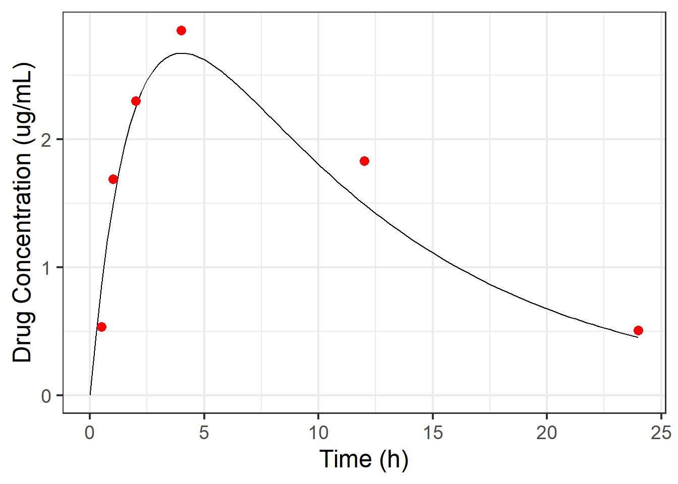
Code
set_cmdstan_path("~/Torsten/cmdstan/")
model_simulate_torsten <- cmdstan_model(
"Torsten/Simulate/depot_1cmt_lognormal_single.stan")
model_simulate_torsten$print()// First Order Absorption (oral/subcutaneous)
// One-compartment PK Model
// Single subject
// lognormal error - DV = CP*exp(eps)
// Closed form solution using a Torsten function
data{
int n_obs;
array[n_obs] real amt;
array[n_obs] int cmt;
array[n_obs] int evid;
array[n_obs] real rate;
array[n_obs] real ii;
array[n_obs] int addl;
array[n_obs] int ss;
array[n_obs] real time;
real<lower = 0> CL;
real<lower = 0> V;
real<lower = CL/V> KA;
real<lower = 0> sigma;
}
model{
}
generated quantities{
vector[n_obs] cp;
vector[n_obs] dv;
{
matrix[n_obs, 2] x_cp;
array[3] real theta_params = {CL, V, KA};
x_cp = pmx_solve_onecpt(time,
amt,
rate,
ii,
evid,
cmt,
addl,
ss,
theta_params)';
cp = x_cp[, 2] ./ V;
}
for(i in 1:n_obs){
if(cp[i] == 0){
dv[i] = 0;
}else{
dv[i] = lognormal_rng(log(cp[i]), sigma);
}
}
}
Code
times_to_observe <- c(0.5, 1, 2, 4, 12, 24)
times_to_simulate <- times_to_observe %>%
c(seq(0.25, 24, by = 0.25)) %>%
sort() %>%
unique()
nonmem_data_single <- mrgsolve::ev(ID = 1, amt = 200, cmt = 1, evid = 1,
rate = 0, ii = 0, addl = 0, ss = 0) %>%
as_tibble() %>%
bind_rows(tibble(ID = 1, time = times_to_simulate, amt = 0, cmt = 2, evid = 0,
rate = 0, ii = 0, addl = 0, ss = 0))
torsten_data_simulate <- with(nonmem_data_single,
list(n_obs = nrow(nonmem_data_single),
amt = amt,
cmt = cmt,
evid = evid,
rate = rate,
ii = ii,
addl = addl,
ss = ss,
time = time,
CL = 5,
V = 50,
KA = 0.5,
sigma = 0.2))
simulated_data_torsten <- model_simulate_torsten$sample(data = torsten_data_simulate,
fixed_param = TRUE,
seed = 1,
iter_warmup = 0,
iter_sampling = 1,
chains = 1,
parallel_chains = 1,
show_messages = TRUE)
data_torsten <- simulated_data_torsten$draws(format = "draws_df") %>%
spread_draws(cp[i], dv[i]) %>%
mutate(time = times_to_simulate[i]) %>%
ungroup() %>%
select(time, cp, dv)
observed_data_torsten <- data_torsten %>%
filter(time %in% times_to_observe) %>%
select(time, dv)Code
observed_data_torsten %>%
mutate(dv = round(dv, 3)) %>%
knitr::kable(col.names = c("Time", "Concentration"),
caption = "Observed Data for a Single Individual") %>%
kableExtra::kable_styling(full_width = FALSE)| Time | Concentration |
|---|---|
| 0.5 | 0.474 |
| 1.0 | 1.668 |
| 2.0 | 2.059 |
| 4.0 | 2.931 |
| 12.0 | 1.502 |
| 24.0 | 0.615 |
And here we can see the observed data overlayed on top of the “truth”.

3.2.3 Fitting the Data
Now we want to fit the data1 to our model. We write the model in a .stan file2 (analogous to a .ctl or .mod file in NONMEM):
I’ve first written a model using pure Stan code. Let’s look at the model.
Code
model_fit_stan <- cmdstan_model(
"Stan/Fit/depot_1cmt_lognormal_single.stan")
model_fit_stan$print()// First Order Absorption (oral/subcutaneous)
// One-compartment PK Model
// Single subject
// lognormal error - DV = CP*exp(eps)
// Closed form solution using a self-written function
functions{
real depot_1cmt(real dose, real cl, real v, real ka,
real time_since_dose){
real ke = cl/v;
real cp = dose/v * ka/(ka - ke) *
(exp(-ke*time_since_dose) - exp(-ka*time_since_dose));
return cp;
}
}
data{
int n_obs;
real<lower = 0> dose;
array[n_obs] real time;
real time_of_first_dose;
vector[n_obs] dv;
real<lower = 0> scale_cl; // Prior Scale parameter for CL
real<lower = 0> scale_v; // Prior Scale parameter for V
real<lower = 0> scale_ka; // Prior Scale parameter for KA
real<lower = 0> scale_sigma; // Prior Scale parameter for lognormal error
int n_pred; // Number of new times at which to make a prediction
array[n_pred] real time_pred; // New times at which to make a prediction
}
transformed data{
vector[n_obs] time_since_dose = to_vector(time) - time_of_first_dose;
vector[n_pred] time_since_dose_pred = to_vector(time_pred) -
time_of_first_dose;
}
parameters{
real<lower = 0> CL;
real<lower = 0> V;
real<lower = CL/V> KA;
real<lower = 0> sigma;
}
transformed parameters{
vector[n_obs] ipred;
for(i in 1:n_obs){
ipred[i] = depot_1cmt(dose, CL, V, KA, time_since_dose[i]);
}
}
model{
// Priors
CL ~ cauchy(0, scale_cl);
V ~ cauchy(0, scale_v);
KA ~ normal(0, scale_ka) T[CL/V, ];
sigma ~ normal(0, scale_sigma);
// Likelihood
dv ~ lognormal(log(ipred), sigma);
}
generated quantities{
real<lower = 0> KE = CL/V;
real<lower = 0> sigma_sq = square(sigma);
vector[n_obs] dv_ppc;
vector[n_obs] log_lik;
vector[n_pred] cp;
vector[n_pred] dv_pred;
vector[n_obs] ires = log(dv) - log(ipred);
vector[n_obs] iwres = ires/sigma;
for(i in 1:n_obs){
dv_ppc[i] = lognormal_rng(log(ipred[i]), sigma);
log_lik[i] = lognormal_lpdf(dv[i] | log(ipred[i]), sigma);
}
for(j in 1:n_pred){
if(time_since_dose_pred[j] <= 0){
cp[j] = 0;
dv_pred[j] = 0;
}else{
cp[j] = depot_1cmt(dose, CL, V, KA, time_since_dose_pred[j]);
dv_pred[j] = lognormal_rng(log(cp[j]), sigma);
}
}
}Now we prepare the data for Stan and fit it:
Code
stan_data_fit <- list(n_obs = nrow(observed_data_torsten),
dose = 200,
time = observed_data_torsten$time,
time_of_first_dose = 0,
dv = observed_data_torsten$dv,
scale_cl = 10,
scale_v = 10,
scale_ka = 1,
scale_sigma = 0.5,
n_pred = length(times_to_simulate),
time_pred = times_to_simulate)
fit_single_stan <- model_fit_stan$sample(data = stan_data_fit,
chains = 4,
# parallel_chains = 4,
iter_warmup = 1000,
iter_sampling = 1000,
adapt_delta = 0.95,
refresh = 500,
max_treedepth = 15,
seed = 8675309,
init = function()
list(CL = rlnorm(1, log(8), 0.3),
V = rlnorm(1, log(40), 0.3),
KA = rlnorm(1, log(0.8), 0.3),
sigma = rlnorm(1, log(0.3), 0.3)))Running MCMC with 4 sequential chains...
Chain 1 Iteration: 1 / 2000 [ 0%] (Warmup)
Chain 1 Iteration: 500 / 2000 [ 25%] (Warmup)
Chain 1 Iteration: 1000 / 2000 [ 50%] (Warmup)
Chain 1 Iteration: 1001 / 2000 [ 50%] (Sampling)
Chain 1 Iteration: 1500 / 2000 [ 75%] (Sampling)
Chain 1 Iteration: 2000 / 2000 [100%] (Sampling)
Chain 1 finished in 0.5 seconds.
Chain 2 Iteration: 1 / 2000 [ 0%] (Warmup)
Chain 2 Iteration: 500 / 2000 [ 25%] (Warmup)
Chain 2 Iteration: 1000 / 2000 [ 50%] (Warmup)
Chain 2 Iteration: 1001 / 2000 [ 50%] (Sampling)
Chain 2 Iteration: 1500 / 2000 [ 75%] (Sampling)
Chain 2 Iteration: 2000 / 2000 [100%] (Sampling)
Chain 2 finished in 0.5 seconds.
Chain 3 Iteration: 1 / 2000 [ 0%] (Warmup)
Chain 3 Iteration: 500 / 2000 [ 25%] (Warmup)
Chain 3 Iteration: 1000 / 2000 [ 50%] (Warmup)
Chain 3 Iteration: 1001 / 2000 [ 50%] (Sampling)
Chain 3 Iteration: 1500 / 2000 [ 75%] (Sampling)
Chain 3 Iteration: 2000 / 2000 [100%] (Sampling)
Chain 3 finished in 0.5 seconds.
Chain 4 Iteration: 1 / 2000 [ 0%] (Warmup)
Chain 4 Iteration: 500 / 2000 [ 25%] (Warmup)
Chain 4 Iteration: 1000 / 2000 [ 50%] (Warmup)
Chain 4 Iteration: 1001 / 2000 [ 50%] (Sampling)
Chain 4 Iteration: 1500 / 2000 [ 75%] (Sampling)
Chain 4 Iteration: 2000 / 2000 [100%] (Sampling)
Chain 4 finished in 0.5 seconds.
All 4 chains finished successfully.
Mean chain execution time: 0.5 seconds.
Total execution time: 2.9 seconds.I’ve now written a model that uses Torsten’s built-in function for a one-compartment PK model. Let’s look at the model.
Code
model_fit_torsten <- cmdstan_model(
"Torsten/Fit/depot_1cmt_lognormal_single.stan")
model_fit_torsten$print()// First Order Absorption (oral/subcutaneous)
// One-compartment PK Model
// Single subject
// lognormal error - DV = CP*exp(eps)
// Closed form solution using a Torsten function
data{
int n_total;
int n_obs;
array[n_obs] int i_obs;
array[n_total] real amt;
array[n_total] int cmt;
array[n_total] int evid;
array[n_total] real rate;
array[n_total] real ii;
array[n_total] int addl;
array[n_total] int ss;
array[n_total] real time;
vector<lower = 0>[n_total] dv;
real<lower = 0> scale_cl; // Prior Scale parameter for CL
real<lower = 0> scale_v; // Prior Scale parameter for V
real<lower = 0> scale_ka; // Prior Scale parameter for KA
real<lower = 0> scale_sigma; // Prior Scale parameter for lognormal error
// These are data variables needed to make predictions at unobserved
// timepoints
int n_pred; // Number of new times at which to make a prediction
array[n_pred] real amt_pred;
array[n_pred] int cmt_pred;
array[n_pred] int evid_pred;
array[n_pred] real rate_pred;
array[n_pred] real ii_pred;
array[n_pred] int addl_pred;
array[n_pred] int ss_pred;
array[n_pred] real time_pred;
}
transformed data{
vector<lower = 0>[n_obs] dv_obs = dv[i_obs];
}
parameters{
real<lower = 0> CL;
real<lower = 0> V;
real<lower = CL/V> KA;
real<lower = 0> sigma;
}
transformed parameters{
vector[n_obs] ipred;
{
vector[n_total] dv_ipred;
matrix[n_total, 2] x_ipred = pmx_solve_onecpt(time,
amt,
rate,
ii,
evid,
cmt,
addl,
ss,
{CL, V, KA})';
dv_ipred = x_ipred[, 2] ./ V;
ipred = dv_ipred[i_obs];
}
}
model{
// Priors
CL ~ cauchy(0, scale_cl);
V ~ cauchy(0, scale_v);
KA ~ normal(0, scale_ka) T[CL/V, ];
sigma ~ normal(0, scale_sigma);
// Likelihood
dv_obs ~ lognormal(log(ipred), sigma);
}
generated quantities{
real<lower = 0> KE = CL/V;
real<lower = 0> sigma_sq = square(sigma);
vector[n_obs] dv_ppc;
vector[n_obs] log_lik;
vector[n_pred] cp;
vector[n_pred] dv_pred;
vector[n_obs] ires = log(dv_obs) - log(ipred);
vector[n_obs] iwres = ires/sigma;
for(i in 1:n_obs){
dv_ppc[i] = lognormal_rng(log(ipred[i]), sigma);
log_lik[i] = lognormal_lpdf(dv[i] | log(ipred[i]), sigma);
}
{
matrix[n_pred, 2] x_cp;
array[3] real theta_params = {CL, V, KA};
x_cp = pmx_solve_onecpt(time_pred,
amt_pred,
rate_pred,
ii_pred,
evid_pred,
cmt_pred,
addl_pred,
ss_pred,
theta_params)';
cp = x_cp[, 2] ./ V;
}
for(i in 1:n_pred){
if(cp[i] == 0){
dv_pred[i] = 0;
}else{
dv_pred[i] = lognormal_rng(log(cp[i]), sigma);
}
}
}
Now we prepare the data for the Stan model with Torsten functions and fit it:
Code
nonmem_data_single_fit <- nonmem_data_single %>%
inner_join(observed_data_torsten, by = "time") %>%
bind_rows(nonmem_data_single %>%
filter(evid == 1)) %>%
arrange(time) %>%
mutate(dv = if_else(is.na(dv), 5555555, dv))
i_obs <- nonmem_data_single_fit %>%
mutate(row_num = 1:n()) %>%
filter(evid == 0) %>%
select(row_num) %>%
deframe()
n_obs <- length(i_obs)
torsten_data_fit <- list(n_total = nrow(nonmem_data_single_fit),
n_obs = n_obs,
i_obs = i_obs,
amt = nonmem_data_single_fit$amt,
cmt = nonmem_data_single_fit$cmt,
evid = nonmem_data_single_fit$evid,
rate = nonmem_data_single_fit$rate,
ii = nonmem_data_single_fit$ii,
addl = nonmem_data_single_fit$addl,
ss = nonmem_data_single_fit$ss,
time = nonmem_data_single_fit$time,
dv = nonmem_data_single_fit$dv,
scale_cl = 10,
scale_v = 10,
scale_ka = 1,
scale_sigma = 0.5,
n_pred = nrow(nonmem_data_single),
amt_pred = nonmem_data_single$amt,
cmt_pred = nonmem_data_single$cmt,
evid_pred = nonmem_data_single$evid,
rate_pred = nonmem_data_single$rate,
ii_pred = nonmem_data_single$ii,
addl_pred = nonmem_data_single$addl,
ss_pred = nonmem_data_single$ss,
time_pred = nonmem_data_single$time)
fit_single_torsten <- model_fit_torsten$sample(data = torsten_data_fit,
chains = 4,
# parallel_chains = 4,
iter_warmup = 1000,
iter_sampling = 1000,
adapt_delta = 0.95,
refresh = 500,
max_treedepth = 15,
seed = 8675309,
init = function()
list(CL = rlnorm(1, log(8), 0.3),
V = rlnorm(1, log(40), 0.3),
KA = rlnorm(1, log(0.8), 0.3),
sigma = rlnorm(1, log(0.3), 0.3)))Running MCMC with 4 sequential chains...
Chain 1 Iteration: 1 / 2000 [ 0%] (Warmup)
Chain 1 Iteration: 500 / 2000 [ 25%] (Warmup)
Chain 1 Iteration: 1000 / 2000 [ 50%] (Warmup)
Chain 1 Iteration: 1001 / 2000 [ 50%] (Sampling)
Chain 1 Iteration: 1500 / 2000 [ 75%] (Sampling)
Chain 1 Iteration: 2000 / 2000 [100%] (Sampling)
Chain 1 finished in 2.8 seconds.
Chain 2 Iteration: 1 / 2000 [ 0%] (Warmup)
Chain 2 Iteration: 500 / 2000 [ 25%] (Warmup)
Chain 2 Iteration: 1000 / 2000 [ 50%] (Warmup)
Chain 2 Iteration: 1001 / 2000 [ 50%] (Sampling)
Chain 2 Iteration: 1500 / 2000 [ 75%] (Sampling)
Chain 2 Iteration: 2000 / 2000 [100%] (Sampling)
Chain 2 finished in 3.8 seconds.
Chain 3 Iteration: 1 / 2000 [ 0%] (Warmup)
Chain 3 Iteration: 500 / 2000 [ 25%] (Warmup)
Chain 3 Iteration: 1000 / 2000 [ 50%] (Warmup)
Chain 3 Iteration: 1001 / 2000 [ 50%] (Sampling)
Chain 3 Iteration: 1500 / 2000 [ 75%] (Sampling)
Chain 3 Iteration: 2000 / 2000 [100%] (Sampling)
Chain 3 finished in 3.3 seconds.
Chain 4 Iteration: 1 / 2000 [ 0%] (Warmup)
Chain 4 Iteration: 500 / 2000 [ 25%] (Warmup)
Chain 4 Iteration: 1000 / 2000 [ 50%] (Warmup)
Chain 4 Iteration: 1001 / 2000 [ 50%] (Sampling)
Chain 4 Iteration: 1500 / 2000 [ 75%] (Sampling)
Chain 4 Iteration: 2000 / 2000 [100%] (Sampling)
Chain 4 finished in 4.0 seconds.
All 4 chains finished successfully.
Mean chain execution time: 3.5 seconds.
Total execution time: 14.6 seconds.3.2.4 Post-Processing and What is Happening
In the post-processing section, we will go through some of the MCMC sampler checking that we should do here, but we will skip it for brevity and go through it more thoroughly later.
We want to look at summaries of the posterior (posterior mean, median, quantiles, and standard deviation), posterior densities for our parameters, and 2D joint posterior densities:
Code
summarize_draws(fit_single_torsten$draws(),
mean, median, sd, mcse_mean,
~quantile2(.x, probs = c(0.025, 0.975)), rhat,
ess_bulk, ess_tail) %>%
mutate(rse = sd/mean*100,
across(where(is.numeric), round, 3)) %>%
select(variable, mean, sd, rse, q2.5, median, q97.5, rhat,
starts_with("ess")) %>%
knitr::kable(col.names = c("Variable", "Mean", "Std. Dev.", "RSE", "2.5%",
"Median", "97.5%", "$\\hat{R}$", "ESS Bulk",
"ESS Tail")) %>%
kableExtra::column_spec(column = 1:10, width = "30em") %>%
kableExtra::scroll_box(width = "800px", height = "200px")| Variable | Mean | Std. Dev. | RSE | 2.5% | Median | 97.5% | $\hat{R}$ | ESS Bulk | ESS Tail |
|---|---|---|---|---|---|---|---|---|---|
| lp__ | -2.137 | 1.798 | -84.121 | -6.661 | -1.756 | 0.246 | 1.008 | 794.635 | 626.653 |
| CL | 4.355 | 1.068 | 24.532 | 1.930 | 4.359 | 6.456 | 1.007 | 980.970 | 440.209 |
| V | 55.489 | 22.499 | 40.546 | 25.248 | 51.614 | 110.525 | 1.006 | 896.816 | 774.931 |
| KA | 0.501 | 0.296 | 59.088 | 0.179 | 0.422 | 1.307 | 1.004 | 1020.112 | 1324.258 |
| sigma | 0.371 | 0.148 | 39.986 | 0.176 | 0.339 | 0.742 | 1.003 | 1084.815 | 1698.531 |
| ipred[1] | 0.754 | 0.207 | 27.408 | 0.469 | 0.719 | 1.248 | 1.001 | 3461.336 | 2169.805 |
| ipred[2] | 1.303 | 0.305 | 23.432 | 0.846 | 1.261 | 2.018 | 1.001 | 3386.615 | 1826.139 |
| ipred[3] | 1.992 | 0.399 | 20.052 | 1.340 | 1.955 | 2.903 | 1.001 | 2202.822 | 1550.524 |
| ipred[4] | 2.490 | 0.505 | 20.283 | 1.542 | 2.475 | 3.576 | 1.001 | 1359.165 | 1227.544 |
| ipred[5] | 1.725 | 0.386 | 22.363 | 1.046 | 1.693 | 2.548 | 1.002 | 1528.417 | 1836.612 |
| ipred[6] | 0.666 | 0.273 | 41.025 | 0.303 | 0.609 | 1.385 | 1.006 | 1125.416 | 521.467 |
| KE | 0.090 | 0.036 | 40.192 | 0.023 | 0.087 | 0.167 | 1.008 | 662.649 | 369.039 |
| sigma_sq | 0.159 | 0.146 | 91.314 | 0.031 | 0.115 | 0.551 | 1.003 | 1084.813 | 1698.531 |
| dv_ppc[1] | 0.820 | 0.524 | 63.912 | 0.303 | 0.714 | 1.948 | 1.001 | 4063.930 | 3293.956 |
| dv_ppc[2] | 1.422 | 0.832 | 58.515 | 0.518 | 1.260 | 3.273 | 1.002 | 3765.599 | 3200.819 |
| dv_ppc[3] | 2.169 | 1.212 | 55.865 | 0.799 | 1.952 | 4.747 | 1.000 | 3722.851 | 2800.842 |
| dv_ppc[4] | 2.729 | 1.402 | 51.371 | 0.970 | 2.489 | 6.261 | 1.001 | 2989.344 | 3079.407 |
| dv_ppc[5] | 1.869 | 1.068 | 57.139 | 0.655 | 1.689 | 4.260 | 1.001 | 3148.926 | 3017.194 |
| dv_ppc[6] | 0.718 | 0.474 | 65.960 | 0.227 | 0.615 | 1.887 | 1.002 | 2113.095 | 1669.165 |
| log_lik[1] | -1376.388 | 1010.713 | -73.432 | -4067.306 | -1112.035 | -235.805 | 1.003 | 1084.735 | 1707.823 |
| log_lik[2] | -4.392 | 3.738 | -85.112 | -14.704 | -3.391 | -0.242 | 1.003 | 1289.555 | 2157.140 |
| log_lik[3] | -0.621 | 0.406 | -65.335 | -1.534 | -0.590 | 0.073 | 1.002 | 1528.992 | 1968.758 |
| log_lik[4] | -0.910 | 0.419 | -46.061 | -1.839 | -0.872 | -0.197 | 1.001 | 1677.842 | 2479.918 |
| log_lik[5] | -2.688 | 1.400 | -52.078 | -6.329 | -2.310 | -1.112 | 1.003 | 1682.743 | 2385.087 |
| log_lik[6] | -5.129 | 4.289 | -83.623 | -16.118 | -3.965 | -0.677 | 1.005 | 1085.823 | 1085.114 |
| cp[1] | 0.000 | 0.000 | NaN | 0.000 | 0.000 | 0.000 | NA | NA | NA |
| cp[2] | 0.407 | 0.123 | 30.280 | 0.246 | 0.384 | 0.709 | 1.001 | 3310.127 | 2035.722 |
| cp[3] | 0.754 | 0.207 | 27.408 | 0.469 | 0.719 | 1.248 | 1.001 | 3461.336 | 2169.805 |
| cp[4] | 1.050 | 0.264 | 25.162 | 0.674 | 1.008 | 1.676 | 1.001 | 3507.971 | 2083.616 |
| cp[5] | 1.303 | 0.305 | 23.432 | 0.846 | 1.261 | 2.018 | 1.001 | 3386.615 | 1826.139 |
| cp[6] | 1.518 | 0.336 | 22.127 | 1.008 | 1.477 | 2.291 | 1.001 | 3120.881 | 1913.441 |
| cp[7] | 1.702 | 0.360 | 21.171 | 1.142 | 1.662 | 2.530 | 1.001 | 2804.595 | 1958.569 |
| cp[8] | 1.859 | 0.381 | 20.498 | 1.257 | 1.822 | 2.723 | 1.001 | 2493.777 | 1976.229 |
| cp[9] | 1.992 | 0.399 | 20.052 | 1.340 | 1.955 | 2.903 | 1.001 | 2202.822 | 1550.524 |
| cp[10] | 2.105 | 0.416 | 19.783 | 1.403 | 2.071 | 3.056 | 1.001 | 1979.723 | 1408.983 |
| cp[11] | 2.199 | 0.432 | 19.652 | 1.455 | 2.168 | 3.166 | 1.001 | 1808.311 | 1262.649 |
| cp[12] | 2.277 | 0.447 | 19.626 | 1.487 | 2.250 | 3.269 | 1.001 | 1678.486 | 1192.524 |
| cp[13] | 2.342 | 0.461 | 19.677 | 1.506 | 2.319 | 3.356 | 1.001 | 1580.388 | 1225.115 |
| cp[14] | 2.394 | 0.474 | 19.783 | 1.524 | 2.372 | 3.438 | 1.001 | 1505.590 | 1266.716 |
| cp[15] | 2.435 | 0.485 | 19.928 | 1.533 | 2.418 | 3.501 | 1.001 | 1444.723 | 1240.637 |
| cp[16] | 2.467 | 0.496 | 20.098 | 1.536 | 2.454 | 3.531 | 1.001 | 1397.028 | 1178.269 |
| cp[17] | 2.490 | 0.505 | 20.283 | 1.542 | 2.475 | 3.576 | 1.001 | 1359.165 | 1227.544 |
| cp[18] | 2.506 | 0.513 | 20.474 | 1.542 | 2.493 | 3.611 | 1.001 | 1330.739 | 1196.487 |
| cp[19] | 2.515 | 0.520 | 20.667 | 1.536 | 2.502 | 3.637 | 1.001 | 1307.819 | 1232.699 |
| cp[20] | 2.519 | 0.525 | 20.856 | 1.527 | 2.506 | 3.628 | 1.001 | 1292.332 | 1274.479 |
| cp[21] | 2.517 | 0.530 | 21.038 | 1.520 | 2.503 | 3.633 | 1.001 | 1283.851 | 1266.188 |
| cp[22] | 2.511 | 0.533 | 21.211 | 1.506 | 2.501 | 3.624 | 1.001 | 1277.842 | 1258.189 |
| cp[23] | 2.500 | 0.534 | 21.373 | 1.491 | 2.492 | 3.613 | 1.001 | 1276.192 | 1362.440 |
| cp[24] | 2.486 | 0.535 | 21.522 | 1.477 | 2.481 | 3.607 | 1.001 | 1276.340 | 1402.978 |
| cp[25] | 2.469 | 0.535 | 21.660 | 1.466 | 2.463 | 3.586 | 1.001 | 1278.436 | 1451.027 |
| cp[26] | 2.450 | 0.534 | 21.784 | 1.454 | 2.444 | 3.552 | 1.001 | 1283.296 | 1442.900 |
| cp[27] | 2.428 | 0.532 | 21.895 | 1.443 | 2.423 | 3.513 | 1.001 | 1288.360 | 1453.902 |
| cp[28] | 2.403 | 0.529 | 21.993 | 1.426 | 2.397 | 3.493 | 1.001 | 1290.774 | 1537.526 |
| cp[29] | 2.377 | 0.525 | 22.078 | 1.412 | 2.369 | 3.453 | 1.001 | 1295.857 | 1615.410 |
| cp[30] | 2.350 | 0.521 | 22.152 | 1.397 | 2.340 | 3.414 | 1.001 | 1301.703 | 1594.963 |
| cp[31] | 2.321 | 0.516 | 22.214 | 1.380 | 2.308 | 3.371 | 1.001 | 1308.465 | 1581.257 |
| cp[32] | 2.291 | 0.510 | 22.265 | 1.366 | 2.274 | 3.328 | 1.001 | 1315.960 | 1571.063 |
| cp[33] | 2.260 | 0.504 | 22.306 | 1.349 | 2.243 | 3.286 | 1.001 | 1323.902 | 1587.716 |
| cp[34] | 2.228 | 0.498 | 22.338 | 1.331 | 2.209 | 3.253 | 1.001 | 1333.695 | 1608.290 |
| cp[35] | 2.196 | 0.491 | 22.362 | 1.310 | 2.175 | 3.198 | 1.001 | 1344.288 | 1641.653 |
| cp[36] | 2.163 | 0.484 | 22.378 | 1.297 | 2.140 | 3.136 | 1.001 | 1354.873 | 1658.188 |
| cp[37] | 2.129 | 0.477 | 22.387 | 1.278 | 2.104 | 3.082 | 1.001 | 1367.972 | 1694.652 |
| cp[38] | 2.095 | 0.469 | 22.392 | 1.260 | 2.069 | 3.027 | 1.001 | 1380.645 | 1710.939 |
| cp[39] | 2.061 | 0.462 | 22.391 | 1.244 | 2.034 | 2.981 | 1.001 | 1396.104 | 1698.673 |
| cp[40] | 2.027 | 0.454 | 22.387 | 1.227 | 2.001 | 2.932 | 1.001 | 1409.412 | 1713.934 |
| cp[41] | 1.993 | 0.446 | 22.380 | 1.206 | 1.965 | 2.885 | 1.001 | 1424.609 | 1736.742 |
| cp[42] | 1.959 | 0.438 | 22.372 | 1.188 | 1.933 | 2.839 | 1.001 | 1440.164 | 1751.570 |
| cp[43] | 1.925 | 0.430 | 22.364 | 1.167 | 1.897 | 2.799 | 1.002 | 1456.632 | 1737.198 |
| cp[44] | 1.891 | 0.423 | 22.356 | 1.143 | 1.861 | 2.756 | 1.002 | 1470.886 | 1777.634 |
| cp[45] | 1.857 | 0.415 | 22.350 | 1.124 | 1.828 | 2.714 | 1.002 | 1482.206 | 1802.901 |
| cp[46] | 1.824 | 0.408 | 22.346 | 1.101 | 1.795 | 2.669 | 1.002 | 1493.578 | 1751.658 |
| cp[47] | 1.791 | 0.400 | 22.347 | 1.081 | 1.760 | 2.615 | 1.002 | 1505.000 | 1759.474 |
| cp[48] | 1.758 | 0.393 | 22.352 | 1.062 | 1.725 | 2.577 | 1.002 | 1516.146 | 1784.567 |
| cp[49] | 1.725 | 0.386 | 22.363 | 1.046 | 1.693 | 2.548 | 1.002 | 1528.417 | 1836.612 |
| cp[50] | 1.693 | 0.379 | 22.382 | 1.026 | 1.660 | 2.500 | 1.002 | 1540.168 | 1776.184 |
| cp[51] | 1.661 | 0.372 | 22.408 | 1.006 | 1.627 | 2.477 | 1.002 | 1551.693 | 1767.806 |
| cp[52] | 1.629 | 0.366 | 22.444 | 0.985 | 1.598 | 2.427 | 1.002 | 1562.940 | 1793.044 |
| cp[53] | 1.598 | 0.359 | 22.490 | 0.966 | 1.565 | 2.389 | 1.002 | 1573.531 | 1768.172 |
| cp[54] | 1.568 | 0.353 | 22.547 | 0.952 | 1.536 | 2.343 | 1.003 | 1583.789 | 1768.061 |
| cp[55] | 1.537 | 0.348 | 22.616 | 0.928 | 1.506 | 2.316 | 1.003 | 1593.857 | 1819.014 |
| cp[56] | 1.508 | 0.342 | 22.697 | 0.910 | 1.478 | 2.277 | 1.003 | 1604.120 | 1836.960 |
| cp[57] | 1.478 | 0.337 | 22.793 | 0.892 | 1.445 | 2.240 | 1.003 | 1611.359 | 1828.081 |
| cp[58] | 1.449 | 0.332 | 22.903 | 0.874 | 1.418 | 2.211 | 1.003 | 1618.564 | 1845.886 |
| cp[59] | 1.421 | 0.327 | 23.028 | 0.858 | 1.389 | 2.183 | 1.003 | 1624.614 | 1819.721 |
| cp[60] | 1.393 | 0.323 | 23.170 | 0.842 | 1.361 | 2.151 | 1.003 | 1629.936 | 1777.485 |
| cp[61] | 1.366 | 0.319 | 23.328 | 0.823 | 1.334 | 2.116 | 1.003 | 1636.732 | 1778.602 |
| cp[62] | 1.339 | 0.315 | 23.503 | 0.806 | 1.307 | 2.079 | 1.004 | 1640.799 | 1604.642 |
| cp[63] | 1.312 | 0.311 | 23.696 | 0.790 | 1.282 | 2.053 | 1.004 | 1643.837 | 1643.536 |
| cp[64] | 1.286 | 0.308 | 23.907 | 0.774 | 1.254 | 2.020 | 1.004 | 1645.462 | 1628.331 |
| cp[65] | 1.261 | 0.304 | 24.136 | 0.756 | 1.229 | 1.983 | 1.004 | 1648.545 | 1685.239 |
| cp[66] | 1.236 | 0.301 | 24.385 | 0.739 | 1.203 | 1.952 | 1.004 | 1648.489 | 1576.650 |
| cp[67] | 1.211 | 0.299 | 24.652 | 0.722 | 1.177 | 1.929 | 1.004 | 1647.030 | 1486.980 |
| cp[68] | 1.187 | 0.296 | 24.939 | 0.705 | 1.154 | 1.899 | 1.004 | 1645.640 | 1420.064 |
| cp[69] | 1.163 | 0.294 | 25.246 | 0.687 | 1.130 | 1.865 | 1.004 | 1642.638 | 1399.048 |
| cp[70] | 1.140 | 0.292 | 25.572 | 0.667 | 1.107 | 1.847 | 1.004 | 1638.386 | 1285.087 |
| cp[71] | 1.117 | 0.290 | 25.917 | 0.654 | 1.082 | 1.819 | 1.004 | 1623.986 | 1208.491 |
| cp[72] | 1.095 | 0.288 | 26.282 | 0.638 | 1.059 | 1.785 | 1.005 | 1595.945 | 1213.554 |
| cp[73] | 1.073 | 0.286 | 26.666 | 0.620 | 1.038 | 1.752 | 1.005 | 1569.831 | 1097.293 |
| cp[74] | 1.052 | 0.285 | 27.070 | 0.602 | 1.015 | 1.731 | 1.005 | 1544.207 | 1024.219 |
| cp[75] | 1.031 | 0.283 | 27.492 | 0.585 | 0.994 | 1.698 | 1.005 | 1524.407 | 988.078 |
| cp[76] | 1.010 | 0.282 | 27.934 | 0.569 | 0.974 | 1.676 | 1.005 | 1497.156 | 942.142 |
| cp[77] | 0.990 | 0.281 | 28.394 | 0.554 | 0.953 | 1.666 | 1.005 | 1475.116 | 962.647 |
| cp[78] | 0.971 | 0.280 | 28.873 | 0.539 | 0.933 | 1.650 | 1.005 | 1454.016 | 922.148 |
| cp[79] | 0.951 | 0.279 | 29.370 | 0.526 | 0.913 | 1.631 | 1.005 | 1432.645 | 858.267 |
| cp[80] | 0.932 | 0.279 | 29.884 | 0.512 | 0.893 | 1.618 | 1.005 | 1409.768 | 820.635 |
| cp[81] | 0.914 | 0.278 | 30.416 | 0.498 | 0.874 | 1.597 | 1.005 | 1387.063 | 786.689 |
| cp[82] | 0.896 | 0.277 | 30.965 | 0.485 | 0.856 | 1.584 | 1.006 | 1365.755 | 754.001 |
| cp[83] | 0.878 | 0.277 | 31.531 | 0.471 | 0.838 | 1.568 | 1.005 | 1346.028 | 659.163 |
| cp[84] | 0.861 | 0.276 | 32.114 | 0.456 | 0.820 | 1.551 | 1.006 | 1323.575 | 637.459 |
| cp[85] | 0.844 | 0.276 | 32.712 | 0.440 | 0.803 | 1.523 | 1.006 | 1304.414 | 638.258 |
| cp[86] | 0.827 | 0.276 | 33.326 | 0.429 | 0.784 | 1.509 | 1.007 | 1287.176 | 579.739 |
| cp[87] | 0.811 | 0.275 | 33.956 | 0.414 | 0.766 | 1.497 | 1.006 | 1270.700 | 573.326 |
| cp[88] | 0.795 | 0.275 | 34.601 | 0.402 | 0.749 | 1.480 | 1.007 | 1252.582 | 569.384 |
| cp[89] | 0.779 | 0.275 | 35.260 | 0.391 | 0.731 | 1.462 | 1.007 | 1237.987 | 579.076 |
| cp[90] | 0.764 | 0.275 | 35.934 | 0.378 | 0.715 | 1.445 | 1.007 | 1221.935 | 578.209 |
| cp[91] | 0.749 | 0.274 | 36.622 | 0.367 | 0.698 | 1.442 | 1.007 | 1207.200 | 561.965 |
| cp[92] | 0.735 | 0.274 | 37.323 | 0.357 | 0.683 | 1.437 | 1.007 | 1192.217 | 557.030 |
| cp[93] | 0.720 | 0.274 | 38.038 | 0.346 | 0.668 | 1.423 | 1.007 | 1177.631 | 545.579 |
| cp[94] | 0.706 | 0.274 | 38.766 | 0.335 | 0.652 | 1.410 | 1.007 | 1165.204 | 544.430 |
| cp[95] | 0.693 | 0.274 | 39.506 | 0.324 | 0.637 | 1.406 | 1.006 | 1151.520 | 524.779 |
| cp[96] | 0.679 | 0.274 | 40.259 | 0.313 | 0.623 | 1.399 | 1.006 | 1139.034 | 522.412 |
| cp[97] | 0.666 | 0.273 | 41.025 | 0.303 | 0.609 | 1.385 | 1.006 | 1125.416 | 521.467 |
| dv_pred[1] | 0.000 | 0.000 | NaN | 0.000 | 0.000 | 0.000 | NA | NA | NA |
| dv_pred[2] | 0.447 | 0.266 | 59.625 | 0.159 | 0.389 | 1.085 | 1.001 | 3818.070 | 2957.421 |
| dv_pred[3] | 0.804 | 0.450 | 55.960 | 0.292 | 0.720 | 1.759 | 1.002 | 3843.261 | 3291.723 |
| dv_pred[4] | 1.135 | 0.699 | 61.579 | 0.393 | 1.015 | 2.640 | 1.000 | 3923.071 | 3046.939 |
| dv_pred[5] | 1.413 | 0.801 | 56.687 | 0.489 | 1.258 | 3.272 | 1.000 | 3927.959 | 2966.367 |
| dv_pred[6] | 1.665 | 1.100 | 66.080 | 0.624 | 1.498 | 3.648 | 1.000 | 3941.923 | 3108.647 |
| dv_pred[7] | 1.858 | 1.235 | 66.450 | 0.720 | 1.662 | 4.104 | 1.001 | 4184.315 | 3265.967 |
| dv_pred[8] | 2.016 | 1.129 | 55.995 | 0.734 | 1.802 | 4.624 | 1.001 | 3870.380 | 2754.671 |
| dv_pred[9] | 2.152 | 1.230 | 57.157 | 0.754 | 1.951 | 4.587 | 1.001 | 3639.027 | 2924.317 |
| dv_pred[10] | 2.315 | 1.960 | 84.658 | 0.819 | 2.080 | 4.983 | 1.000 | 3872.531 | 3057.195 |
| dv_pred[11] | 2.406 | 1.619 | 67.306 | 0.866 | 2.161 | 5.262 | 1.000 | 3624.962 | 2850.676 |
| dv_pred[12] | 2.443 | 1.262 | 51.682 | 0.874 | 2.244 | 5.293 | 1.000 | 3141.947 | 2718.986 |
| dv_pred[13] | 2.532 | 1.465 | 57.850 | 0.899 | 2.318 | 5.533 | 1.001 | 3364.679 | 2789.529 |
| dv_pred[14] | 2.603 | 1.440 | 55.327 | 0.927 | 2.381 | 5.679 | 1.001 | 3435.816 | 3177.955 |
| dv_pred[15] | 2.678 | 1.644 | 61.384 | 0.940 | 2.425 | 5.831 | 1.001 | 2767.301 | 2814.226 |
| dv_pred[16] | 2.668 | 1.457 | 54.582 | 0.933 | 2.445 | 5.660 | 1.000 | 2908.415 | 2344.151 |
| dv_pred[17] | 2.689 | 1.372 | 51.007 | 0.961 | 2.459 | 6.012 | 1.000 | 2959.315 | 2660.712 |
| dv_pred[18] | 2.748 | 1.618 | 58.879 | 0.960 | 2.478 | 5.981 | 1.002 | 2959.956 | 2526.857 |
| dv_pred[19] | 2.712 | 1.381 | 50.912 | 0.964 | 2.469 | 6.082 | 1.001 | 2561.149 | 2693.410 |
| dv_pred[20] | 2.760 | 1.486 | 53.850 | 0.973 | 2.508 | 5.980 | 1.000 | 3038.825 | 3001.176 |
| dv_pred[21] | 2.716 | 1.423 | 52.374 | 0.990 | 2.471 | 5.859 | 1.000 | 3005.574 | 2681.790 |
| dv_pred[22] | 2.725 | 1.392 | 51.082 | 0.948 | 2.485 | 5.887 | 1.001 | 2759.230 | 2728.163 |
| dv_pred[23] | 2.688 | 1.329 | 49.441 | 0.939 | 2.481 | 5.703 | 1.001 | 2908.465 | 3197.180 |
| dv_pred[24] | 2.710 | 1.438 | 53.054 | 0.930 | 2.479 | 5.849 | 1.000 | 2653.094 | 2828.734 |
| dv_pred[25] | 2.695 | 1.552 | 57.601 | 0.901 | 2.468 | 5.762 | 1.001 | 3026.305 | 2909.133 |
| dv_pred[26] | 2.676 | 1.447 | 54.080 | 0.908 | 2.434 | 5.769 | 1.000 | 2895.777 | 2734.100 |
| dv_pred[27] | 2.626 | 1.365 | 51.983 | 0.925 | 2.397 | 5.762 | 1.001 | 2890.257 | 2802.849 |
| dv_pred[28] | 2.577 | 1.368 | 53.088 | 0.936 | 2.344 | 5.662 | 1.001 | 2797.384 | 2698.817 |
| dv_pred[29] | 2.574 | 1.431 | 55.607 | 0.851 | 2.331 | 5.516 | 1.000 | 2870.321 | 2939.255 |
| dv_pred[30] | 2.519 | 1.287 | 51.087 | 0.809 | 2.317 | 5.444 | 1.001 | 2657.040 | 2702.597 |
| dv_pred[31] | 2.547 | 1.631 | 64.032 | 0.870 | 2.285 | 5.755 | 1.001 | 2524.845 | 2924.445 |
| dv_pred[32] | 2.497 | 1.305 | 52.270 | 0.843 | 2.268 | 5.437 | 1.002 | 2269.055 | 2652.609 |
| dv_pred[33] | 2.430 | 1.278 | 52.598 | 0.783 | 2.212 | 5.297 | 1.002 | 2806.445 | 2925.347 |
| dv_pred[34] | 2.432 | 1.470 | 60.451 | 0.808 | 2.236 | 5.162 | 1.002 | 2789.945 | 2688.141 |
| dv_pred[35] | 2.391 | 2.861 | 119.671 | 0.778 | 2.155 | 5.236 | 1.000 | 2483.533 | 2763.568 |
| dv_pred[36] | 2.325 | 1.168 | 50.239 | 0.795 | 2.143 | 5.192 | 1.001 | 2775.385 | 2890.691 |
| dv_pred[37] | 2.307 | 1.166 | 50.533 | 0.748 | 2.102 | 4.904 | 1.001 | 2751.990 | 2824.307 |
| dv_pred[38] | 2.264 | 1.166 | 51.498 | 0.743 | 2.059 | 4.990 | 1.000 | 2776.428 | 2570.533 |
| dv_pred[39] | 2.239 | 1.219 | 54.425 | 0.725 | 2.041 | 5.031 | 1.001 | 2669.571 | 2681.213 |
| dv_pred[40] | 2.172 | 1.040 | 47.879 | 0.742 | 1.983 | 4.706 | 1.002 | 2574.518 | 2963.137 |
| dv_pred[41] | 2.157 | 1.368 | 63.422 | 0.723 | 1.966 | 4.655 | 1.002 | 2678.576 | 2785.044 |
| dv_pred[42] | 2.139 | 1.155 | 54.012 | 0.716 | 1.940 | 4.806 | 1.001 | 2875.284 | 2896.157 |
| dv_pred[43] | 2.097 | 1.181 | 56.328 | 0.704 | 1.897 | 4.638 | 1.000 | 2581.940 | 2493.340 |
| dv_pred[44] | 2.046 | 1.064 | 52.020 | 0.718 | 1.861 | 4.500 | 1.000 | 2451.147 | 3136.163 |
| dv_pred[45] | 2.019 | 1.053 | 52.170 | 0.708 | 1.828 | 4.444 | 1.000 | 3238.931 | 3281.057 |
| dv_pred[46] | 1.949 | 0.969 | 49.713 | 0.669 | 1.795 | 4.373 | 1.001 | 2896.901 | 2754.905 |
| dv_pred[47] | 1.927 | 1.032 | 53.575 | 0.649 | 1.745 | 4.134 | 1.002 | 2863.391 | 2765.566 |
| dv_pred[48] | 1.913 | 1.002 | 52.398 | 0.690 | 1.726 | 4.194 | 1.001 | 2635.603 | 2999.175 |
| dv_pred[49] | 1.886 | 1.175 | 62.274 | 0.658 | 1.697 | 4.143 | 1.000 | 3218.694 | 2735.446 |
| dv_pred[50] | 1.836 | 1.115 | 60.714 | 0.642 | 1.651 | 4.131 | 1.002 | 3100.467 | 3110.115 |
| dv_pred[51] | 1.801 | 0.966 | 53.655 | 0.637 | 1.633 | 3.945 | 1.001 | 2979.938 | 2768.123 |
| dv_pred[52] | 1.748 | 0.939 | 53.733 | 0.577 | 1.589 | 4.008 | 1.000 | 2551.083 | 2835.196 |
| dv_pred[53] | 1.764 | 1.103 | 62.507 | 0.601 | 1.577 | 3.935 | 1.002 | 3189.534 | 3284.027 |
| dv_pred[54] | 1.699 | 1.004 | 59.119 | 0.599 | 1.536 | 3.783 | 1.002 | 3036.695 | 3297.585 |
| dv_pred[55] | 1.668 | 0.864 | 51.833 | 0.587 | 1.514 | 3.693 | 1.001 | 2899.314 | 3047.590 |
| dv_pred[56] | 1.641 | 0.844 | 51.446 | 0.586 | 1.475 | 3.639 | 1.000 | 3112.393 | 2624.276 |
| dv_pred[57] | 1.611 | 0.882 | 54.741 | 0.585 | 1.463 | 3.605 | 1.000 | 3139.052 | 3347.912 |
| dv_pred[58] | 1.572 | 0.827 | 52.637 | 0.538 | 1.415 | 3.515 | 1.000 | 2895.760 | 3023.591 |
| dv_pred[59] | 1.547 | 0.899 | 58.113 | 0.529 | 1.402 | 3.478 | 1.001 | 2849.552 | 2984.601 |
| dv_pred[60] | 1.518 | 0.850 | 55.979 | 0.556 | 1.356 | 3.523 | 1.002 | 2945.537 | 2982.626 |
| dv_pred[61] | 1.478 | 0.825 | 55.859 | 0.529 | 1.330 | 3.346 | 1.001 | 3464.706 | 3008.463 |
| dv_pred[62] | 1.474 | 0.851 | 57.749 | 0.518 | 1.315 | 3.293 | 1.002 | 2399.661 | 3133.712 |
| dv_pred[63] | 1.418 | 0.807 | 56.941 | 0.514 | 1.275 | 3.252 | 1.001 | 2867.998 | 2951.121 |
| dv_pred[64] | 1.388 | 0.801 | 57.697 | 0.493 | 1.253 | 3.212 | 1.001 | 2946.870 | 2750.863 |
| dv_pred[65] | 1.371 | 0.713 | 51.970 | 0.484 | 1.247 | 3.098 | 1.001 | 3029.518 | 2766.086 |
| dv_pred[66] | 1.369 | 0.966 | 70.506 | 0.473 | 1.218 | 3.195 | 1.002 | 3153.732 | 2654.869 |
| dv_pred[67] | 1.310 | 0.777 | 59.357 | 0.447 | 1.163 | 2.969 | 1.002 | 3008.766 | 2682.113 |
| dv_pred[68] | 1.314 | 0.763 | 58.070 | 0.434 | 1.175 | 3.176 | 1.001 | 2801.894 | 2580.734 |
| dv_pred[69] | 1.248 | 0.758 | 60.711 | 0.438 | 1.131 | 2.799 | 1.001 | 3022.266 | 2021.036 |
| dv_pred[70] | 1.236 | 0.697 | 56.347 | 0.432 | 1.106 | 2.882 | 1.000 | 3047.656 | 2688.365 |
| dv_pred[71] | 1.199 | 0.703 | 58.614 | 0.419 | 1.075 | 2.675 | 1.001 | 3070.487 | 2440.910 |
| dv_pred[72] | 1.168 | 0.661 | 56.571 | 0.397 | 1.054 | 2.715 | 1.001 | 2964.047 | 2496.541 |
| dv_pred[73] | 1.175 | 0.727 | 61.888 | 0.403 | 1.037 | 2.756 | 1.001 | 2759.395 | 2378.120 |
| dv_pred[74] | 1.147 | 0.636 | 55.400 | 0.380 | 1.024 | 2.669 | 1.002 | 2609.560 | 1751.163 |
| dv_pred[75] | 1.147 | 1.181 | 102.950 | 0.352 | 1.001 | 2.733 | 1.002 | 2838.048 | 2265.052 |
| dv_pred[76] | 1.094 | 0.607 | 55.514 | 0.386 | 0.976 | 2.431 | 1.000 | 2898.406 | 2367.640 |
| dv_pred[77] | 1.073 | 0.605 | 56.428 | 0.353 | 0.952 | 2.598 | 1.004 | 2517.548 | 1849.124 |
| dv_pred[78] | 1.045 | 0.615 | 58.835 | 0.348 | 0.930 | 2.419 | 1.002 | 3078.508 | 2414.908 |
| dv_pred[79] | 1.030 | 0.642 | 62.325 | 0.343 | 0.908 | 2.457 | 1.002 | 2842.938 | 2372.292 |
| dv_pred[80] | 1.016 | 0.663 | 65.204 | 0.338 | 0.892 | 2.491 | 1.001 | 2522.017 | 2042.289 |
| dv_pred[81] | 0.988 | 0.731 | 73.932 | 0.325 | 0.864 | 2.486 | 1.002 | 2343.766 | 1934.742 |
| dv_pred[82] | 0.984 | 0.770 | 78.300 | 0.327 | 0.852 | 2.402 | 1.002 | 2478.733 | 1501.345 |
| dv_pred[83] | 0.964 | 0.669 | 69.449 | 0.317 | 0.838 | 2.341 | 1.001 | 2987.248 | 2264.714 |
| dv_pred[84] | 0.921 | 0.540 | 58.685 | 0.301 | 0.815 | 2.187 | 1.003 | 2557.602 | 2063.966 |
| dv_pred[85] | 0.917 | 0.586 | 63.869 | 0.298 | 0.797 | 2.309 | 1.003 | 2567.302 | 2507.972 |
| dv_pred[86] | 0.900 | 0.581 | 64.528 | 0.305 | 0.784 | 2.180 | 1.003 | 2752.548 | 1796.800 |
| dv_pred[87] | 0.884 | 0.876 | 99.088 | 0.285 | 0.754 | 2.198 | 1.003 | 2414.141 | 1951.958 |
| dv_pred[88] | 0.861 | 0.590 | 68.583 | 0.284 | 0.744 | 2.103 | 1.002 | 2202.549 | 1522.078 |
| dv_pred[89] | 0.844 | 0.515 | 61.053 | 0.287 | 0.728 | 2.112 | 1.001 | 2527.825 | 1930.587 |
| dv_pred[90] | 0.822 | 0.535 | 65.106 | 0.268 | 0.716 | 2.079 | 1.003 | 1804.574 | 1470.038 |
| dv_pred[91] | 0.809 | 0.543 | 67.127 | 0.245 | 0.702 | 2.011 | 1.002 | 2761.356 | 1656.639 |
| dv_pred[92] | 0.810 | 0.713 | 88.048 | 0.249 | 0.684 | 2.079 | 1.002 | 2117.533 | 1880.745 |
| dv_pred[93] | 0.784 | 0.501 | 63.936 | 0.240 | 0.664 | 2.043 | 1.002 | 2115.718 | 1632.866 |
| dv_pred[94] | 0.776 | 0.574 | 73.969 | 0.238 | 0.660 | 2.057 | 1.003 | 1907.815 | 1368.044 |
| dv_pred[95] | 0.763 | 0.719 | 94.317 | 0.235 | 0.646 | 1.989 | 1.003 | 1914.341 | 1561.765 |
| dv_pred[96] | 0.746 | 0.544 | 73.010 | 0.218 | 0.635 | 2.004 | 1.004 | 1606.362 | 1149.605 |
| dv_pred[97] | 0.725 | 0.518 | 71.512 | 0.205 | 0.607 | 2.011 | 1.003 | 1842.228 | 1037.075 |
| ires[1] | -0.434 | 0.240 | -55.298 | -0.969 | -0.418 | 0.010 | 1.001 | 3461.309 | 2169.805 |
| ires[2] | 0.271 | 0.212 | 78.353 | -0.190 | 0.280 | 0.679 | 1.001 | 3386.622 | 1826.139 |
| ires[3] | 0.051 | 0.190 | 369.214 | -0.343 | 0.052 | 0.430 | 1.002 | 2202.833 | 1550.524 |
| ires[4] | 0.184 | 0.205 | 111.721 | -0.199 | 0.169 | 0.642 | 1.001 | 1359.157 | 1227.544 |
| ires[5] | -0.114 | 0.225 | -198.597 | -0.528 | -0.120 | 0.362 | 1.002 | 1528.414 | 1836.612 |
| ires[6] | -0.011 | 0.367 | -3341.167 | -0.812 | 0.010 | 0.708 | 1.005 | 1125.416 | 521.467 |
| iwres[1] | -1.303 | 0.712 | -54.614 | -2.798 | -1.275 | 0.020 | 1.001 | 2163.697 | 2827.847 |
| iwres[2] | 0.861 | 0.646 | 75.064 | -0.358 | 0.841 | 2.161 | 1.001 | 2238.880 | 1976.552 |
| iwres[3] | 0.157 | 0.477 | 304.638 | -0.777 | 0.159 | 1.070 | 1.000 | 3015.700 | 2458.927 |
| iwres[4] | 0.538 | 0.536 | 99.688 | -0.454 | 0.512 | 1.629 | 1.000 | 1996.959 | 2733.015 |
| iwres[5] | -0.378 | 0.647 | -171.053 | -1.669 | -0.352 | 0.815 | 1.002 | 1617.519 | 2248.742 |
| iwres[6] | 0.004 | 0.946 | 21979.166 | -1.849 | 0.032 | 1.849 | 1.004 | 1529.114 | 1270.987 |
Code
mcmc_pairs(fit_single_torsten$draws(c("CL", "V", "KA", "sigma")),
diag_fun = "dens")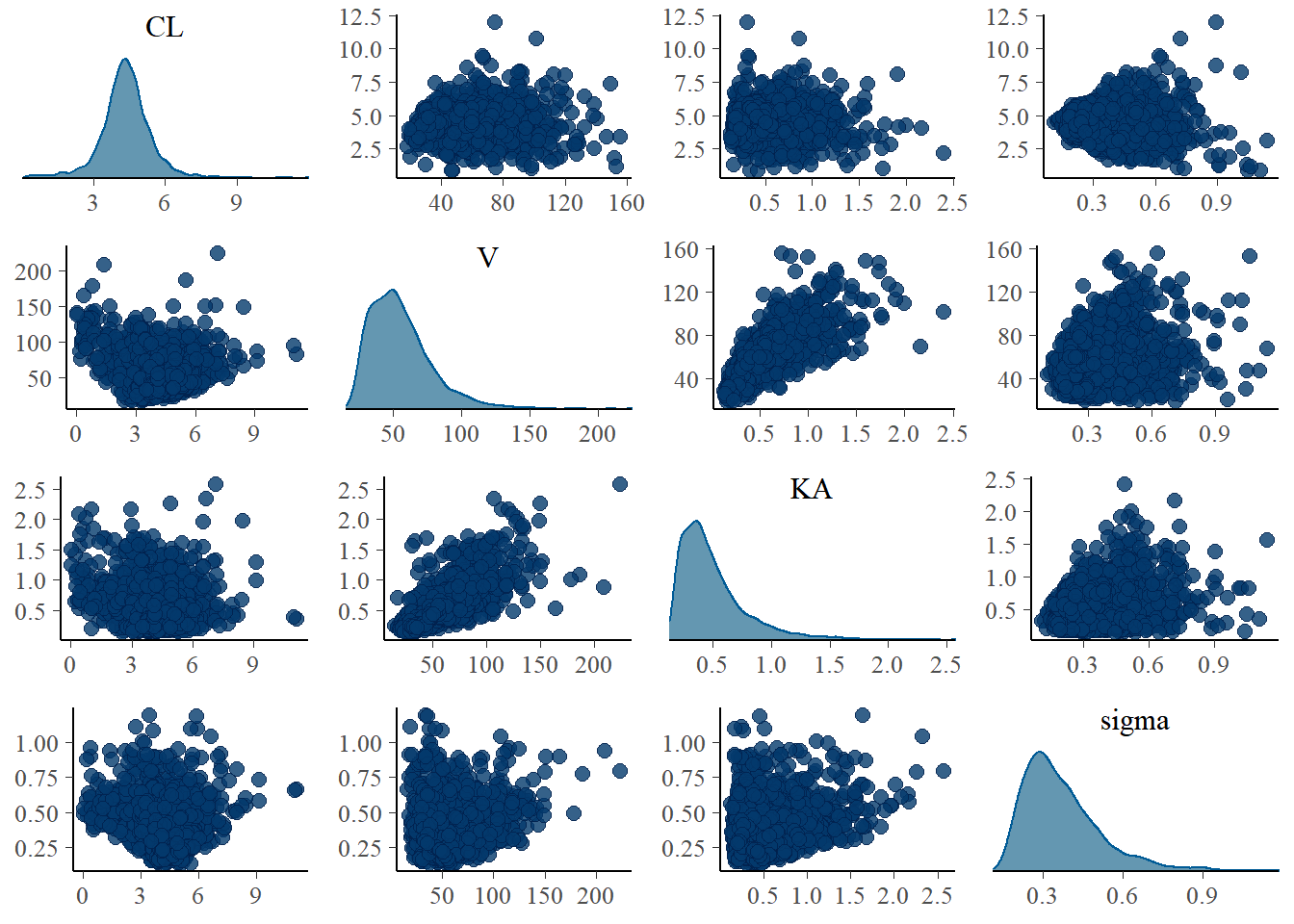
We have also created a predicted curve for each draw from the posterior ( cp in the code). Here, 5 draws are highlighted, and you can see the curve corresponding to each of these draws, along with a few others:
Code
draws_single <- fit_single_torsten$draws(format = "draws_df")
draws_to_highlight <- seq(1, 9, by = 2)
colors_to_highlight <- c("red", "blue", "green", "purple", "orange")
draws_single %>%
filter(.draw <= 100) %>%
select(starts_with("."), CL, V, KA, KE, sigma, starts_with(c("cp", "dv"))) %>%
as_tibble() %>%
mutate(across(where(is.double), round, 3)) %>%
DT::datatable(rownames = FALSE, filter = "top",
options = list(scrollX = TRUE,
columnDefs = list(list(className = 'dt-center',
targets = "_all")))) %>%
DT::formatStyle(".draw", target = "row",
backgroundColor = DT::styleEqual(draws_to_highlight,
colors_to_highlight))Code
preds_single <- draws_single %>%
spread_draws(cp[i], dv_pred[i]) %>%
mutate(time = torsten_data_fit$time_pred[i]) %>%
ungroup() %>%
arrange(.draw, time)
preds_single %>%
mutate(sample_draws = .draw %in% draws_to_highlight,
color = case_when(.draw == draws_to_highlight[1] ~
colors_to_highlight[1],
.draw == draws_to_highlight[2] ~
colors_to_highlight[2],
.draw == draws_to_highlight[3] ~
colors_to_highlight[3],
.draw == draws_to_highlight[4] ~
colors_to_highlight[4],
.draw == draws_to_highlight[5] ~
colors_to_highlight[5],
TRUE ~ "black")) %>%
# filter(.draw %in% c(draws_to_highlight, sample(11:max(.draw), 100))) %>%
filter(.draw <= 100) %>%
arrange(desc(.draw)) %>%
ggplot(aes(x = time, y = cp, group = .draw)) +
geom_line(aes(size = sample_draws, alpha = sample_draws, color = color),
show.legend = FALSE) +
scale_color_manual(name = NULL,
breaks = c("red", "blue", "green", "purple", "orange",
"black"),
values = c("red", "blue", "green", "purple", "orange",
"black")) +
scale_size_manual(name = NULL,
breaks = c(FALSE, TRUE),
values = c(1, 1.5)) +
scale_alpha_manual(name = NULL,
breaks = c(FALSE, TRUE),
values = c(0.10, 1)) +
theme_bw(20) +
scale_x_continuous(name = "Time (h)") +
scale_y_continuous(name = "Drug Concentration (ug/mL)")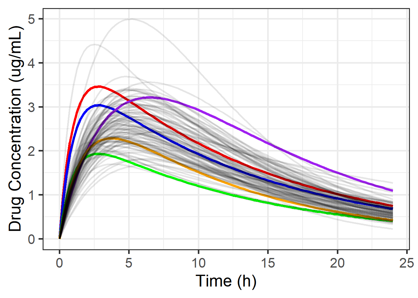
This collection of predicted concentration curves, one for each sample from the posterior distribution, gives us a distribution for the “true” concentration at each time point. From this distribution we can plot our mean prediction (essentially an IPRED curve) and 95% credible interval (the Bayesian version of a confidence interval) for that mean:
Code
(mean_and_ci <- preds_single %>%
group_by(time) %>%
mean_qi(cp, .width = 0.95) %>%
ggplot(aes(x = time, y = cp)) +
geom_line(size = 1.5) +
geom_ribbon(aes(ymin = .lower, ymax = .upper),
fill = "yellow", alpha = 0.25) +
theme_bw(20) +
scale_x_continuous(name = "Time (h)") +
scale_y_continuous(name = "Drug Concentration (ug/mL)") +
coord_cartesian(ylim = c(0, 4.5)))
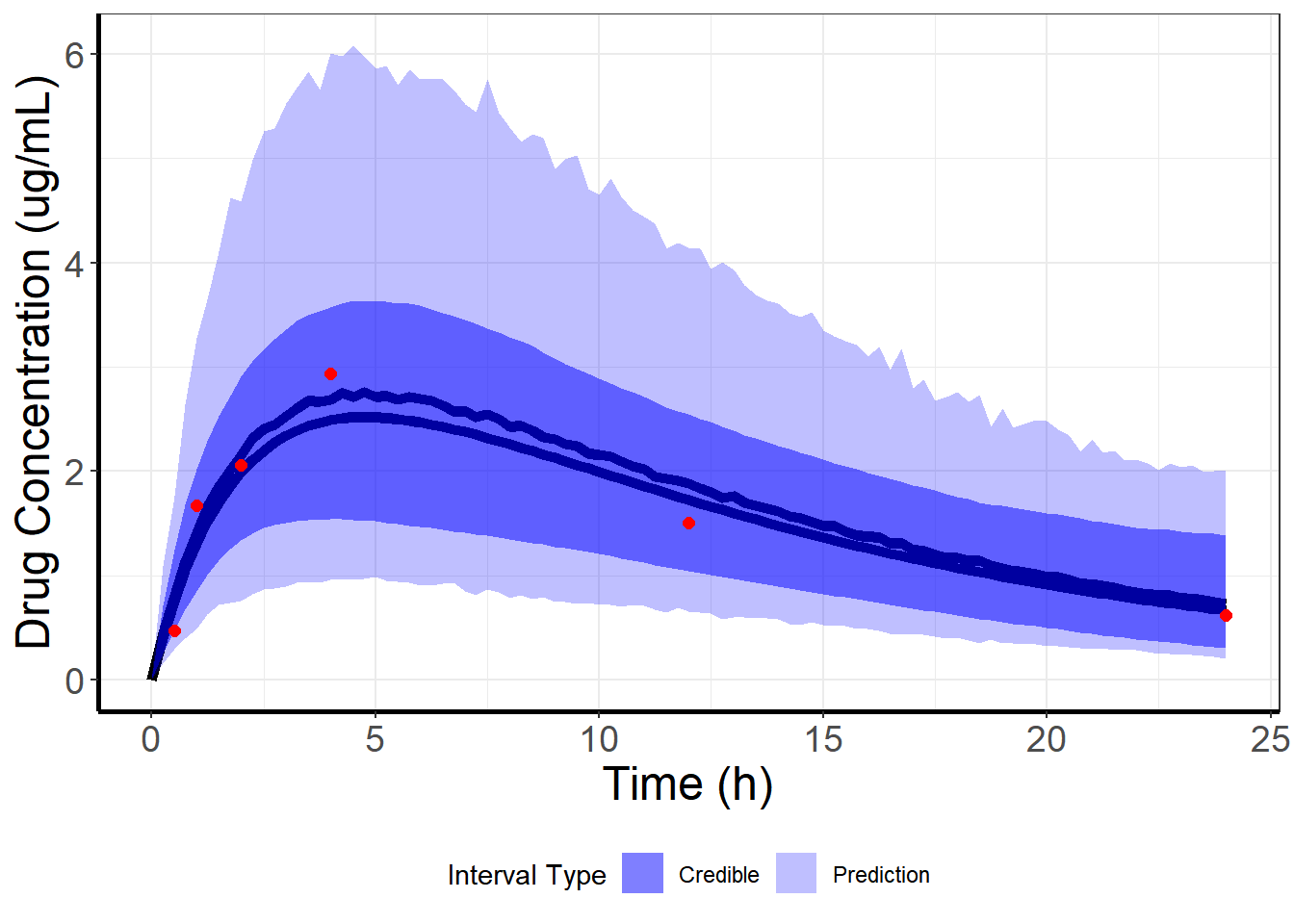
To do some model checking and to make future predictions, we can also get a mean prediction and 95% prediction interval from our replicates of the concentration (one replicate, dv, for each draw from the posterior):
Code
(mean_and_pi <- preds_single %>%
group_by(time) %>%
mean_qi(dv_pred, .width = 0.95) %>%
ggplot(aes(x = time, y = dv_pred)) +
geom_line(size = 1.5) +
geom_ribbon(aes(ymin = .lower, ymax = .upper),
fill = "yellow", alpha = 0.25) +
theme_bw(20) +
scale_x_continuous(name = "Time (h)") +
scale_y_continuous(name = "Drug Concentration (ug/mL)") +
coord_cartesian(ylim = c(0, 6)))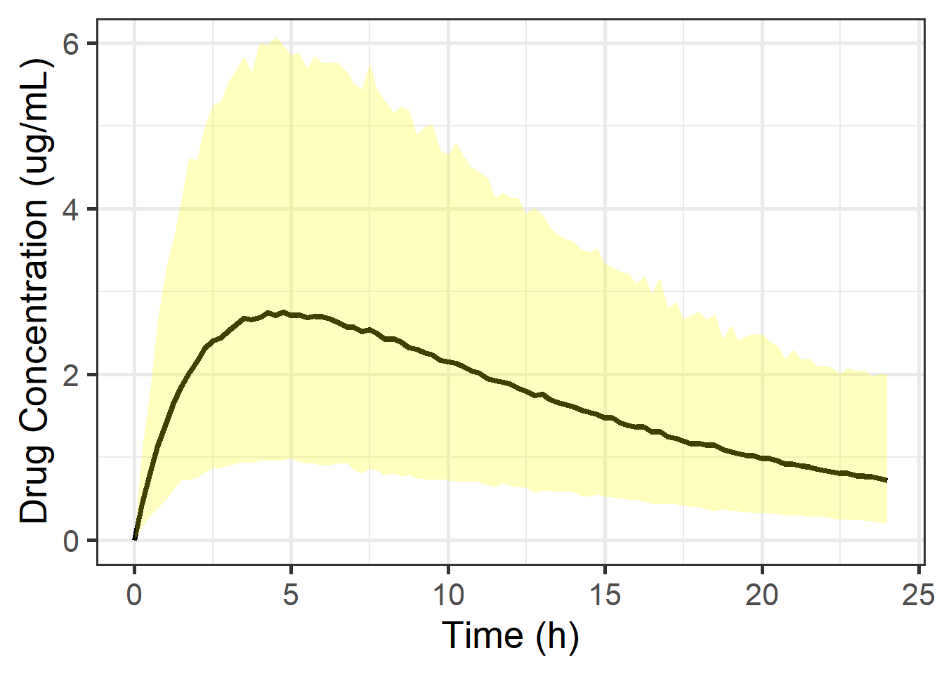
What’s actually happening is that we get the posterior density of the prediction for a given time3

Let’s look at the posterior density for the time points that were actually observed:
Code
mean_and_pi +
stat_halfeye(data = preds_single %>%
filter(time %in% times_to_observe),
aes(x = time, y = dv_pred, group = time),
scale = 2, interval_size = 2, .width = 0.95,
point_interval = mean_qi, normalize = "xy") +
geom_point(data = observed_data_torsten,
mapping = aes(x = time, y = dv), color = "red", size = 3) +
coord_cartesian(ylim = c(0, 6))
3.3 Two-Compartment Model with IV Infusion
We will use a simple, easily understood, and commonly used model to show many of the elements of the workflow of PopPK modeling in Stan with Torsten. We will talk about
- Simulation
- Methods for selection of priors
- Handling BLOQ values
- Prediction for observed subjects and potential future patients
- Covariate effects
- Within-Chain parallelization to speed up the MCMC sampling
3.3.1 PK Model
In this example I have simulated data from a two-compartment model with IV infusion with proportional-plus-additive error. The data-generating model is \[C_{ij} = f(\mathbf{\theta}_i, t_{ij})*\left( 1 + \epsilon_{p_{ij}} \right) + \epsilon_{a_{ij}}\] where \(\mathbf{\theta}_i = \left[CL_i, \, V_{c_i}, \, Q_i, \,V_{p_i}\right]^\top\) is a vector containing the individual parameters for individual \(i\)4, and \(f(\cdot, \cdot)\) is the two-compartment model mean function seen here. The corresponding system of ODEs is:
\[\begin{align} \frac{dA_d}{dt} &= -K_a*A_d \notag \\ \frac{dA_c}{dt} &= rate_{in} + K_a*A_d - \left(\frac{CL}{V_c} + \frac{Q}{V_c}\right)A_C + \frac{Q}{V_p}A_p \notag \\ \frac{dA_p}{dt} &= \frac{Q}{V_c}A_c - \frac{Q}{V_p}A_p \\ \end{align} \tag{3.1}\]
and then \(C = \frac{A_c}{V_c}\)5.
The true parameters used to simulate the data are as follows:
| Parameter | Value | Units | Description |
|---|---|---|---|
| TVCL | 0.20 | \(\frac{L}{d}\) | Population value for clearance |
| TVVC | 3.00 | \(L\) | Population value for central compartment volume |
| TVQ | 1.40 | \(\frac{L}{d}\) | Population value for intercompartmental clearance |
| TVVP | 4.00 | \(L\) | Population value for peripheral compartment volume |
| \(\omega_{CL}\) | 0.30 | - | Standard deviation for IIV in \(CL\) |
| \(\omega_{V_c}\) | 0.25 | - | Standard deviation for IIV in \(V_c\) |
| \(\omega_{Q}\) | 0.20 | - | Standard deviation for IIV in \(Q\) |
| \(\omega_{V_p}\) | 0.15 | - | Standard deviation for IIV in \(V_p\) |
| \(\rho_{CL,V_c}\) | 0.10 | - | Correlation between \(\eta_{CL}\) and \(\eta_{V_c}\) |
| \(\rho_{CL,Q}\) | 0.00 | - | Correlation between \(\eta_{CL}\) and \(\eta_{Q}\) |
| \(\rho_{CL,V_p}\) | 0.10 | - | Correlation between \(\eta_{CL}\) and \(\eta_{V_p}\) |
| \(\rho_{V_c,Q}\) | -0.10 | - | Correlation between \(\eta_{V_c}\) and \(\eta_{Q}\) |
| \(\rho_{V_c,V_p}\) | 0.20 | - | Correlation between \(\eta_{V_c}\) and \(\eta_{V_p}\) |
| \(\rho_{Q,V_p}\) | 0.15 | - | Correlation between \(\eta_{Q}\) and \(\eta_{V_p}\) |
| \(\sigma_p\) | 0.20 | - | Standard deviation for proportional residual error |
| \(\sigma_a\) | 0.03 | \(\frac{\mu g}{mL}\) | Standard deviation for additive residual error |
| \(\rho_{p,a}\) | 0.00 | - | Correlation between \(\epsilon_p\) and \(\epsilon_a\) |
3.3.2 Statistical Model
I’ll write down two models that are very similar with the only differences being the prior distributions on the population parameters.
In the interest of thoroughness and completeness, I’ll write down the full statistical model. For this presentation, I’ll just fit the data to the data-generating model. Letting \[\begin{align} \Omega &= \begin{pmatrix} \omega^2_{CL} & \omega_{CL, V_c} & \omega_{CL, Q} & \omega_{CL, V_p} \\ \omega_{CL, V_c} & \omega^2_{V_c} & \omega_{V_c, Q} & \omega_{V_c, V_p} \\ \omega_{CL, Q} & \omega_{V_c, Q} & \omega^2_{Q} & \omega_{Q, V_p} \\ \omega_{CL, V_p} & \omega_{V_c, V_p} & \omega_{Q, V_p} & \omega^2_{V_p} \\ \end{pmatrix} \\ &= \begin{pmatrix} \omega_{CL} & 0 & 0 & 0 \\ 0 & \omega_{V_c} & 0 & 0 \\ 0 & 0 & \omega_{Q} & 0 \\ 0 & 0 & 0 & \omega_{V_p} \\ \end{pmatrix} \mathbf{R_{\Omega}} \begin{pmatrix} \omega_{CL} & 0 & 0 & 0 \\ 0 & \omega_{V_c} & 0 & 0 \\ 0 & 0 & \omega_{Q} & 0 \\ 0 & 0 & 0 & \omega_{V_p} \\ \end{pmatrix} \\ &= \begin{pmatrix} \omega_{CL} & 0 & 0 & 0 \\ 0 & \omega_{V_c} & 0 & 0 \\ 0 & 0 & \omega_{Q} & 0 \\ 0 & 0 & 0 & \omega_{V_p} \\ \end{pmatrix} \begin{pmatrix} 1 & \rho_{CL, V_c} & \rho_{CL, Q} & \rho_{CL, V_p} \\ \rho_{CL, V_c} & 1 & \rho_{V_c, Q} & \rho_{V_c, V_p} \\ \rho_{CL, Q} & \rho_{V_c, Q} & 1 & \rho_{Q, V_p} \\ \rho_{CL, V_p} & \rho_{V_c, V_p} & \rho_{Q, V_p} & 1 \\ \end{pmatrix} \begin{pmatrix} \omega_{CL} & 0 & 0 & 0 \\ 0 & \omega_{V_c} & 0 & 0 \\ 0 & 0 & \omega_{Q} & 0 \\ 0 & 0 & 0 & \omega_{V_p} \\ \end{pmatrix} \end{align}\] I’ll model the correlation matrix \(R_{\Omega}\) and standard deviations (\(\omega_p\)) of the random effects rather than the covariance matrix \(\Omega\) that is typically done in NONMEM. The full statistical model is \[\begin{align} C_{ij} \mid \mathbf{TV}, \; \mathbf{\eta}_i, \; \mathbf{\Omega}, \; \mathbf{\Sigma} &\sim Normal\left( f(\mathbf{\theta}_i, t_{ij}), \; \sigma_{ij} \right) I(C_{ij} > 0) \notag \\ \mathbf{\eta}_i \; | \; \Omega &\sim Normal\left( \begin{pmatrix} 0 \\ 0 \\ 0 \\ 0 \\ \end{pmatrix} , \; \Omega\right) \notag \\ TVCL &\sim Half-Cauchy\left(0, scale_{TVCL}\right) \notag \\ TVVC &\sim Half-Cauchy\left(0, scale_{TVVC}\right) \notag \\ TVQ &\sim Half-Cauchy\left(0, scale_{TVQ}\right) \notag \\ TVVP &\sim Half-Cauchy\left(0, scale_{TVVP}\right) \notag \\ \omega_{CL} &\sim Half-Normal(0, scale_{\omega_{CL}}) \notag \\ \omega_{V_c} &\sim Half-Normal(0, scale_{\omega_{V_c}}) \notag \\ \omega_{Q} &\sim Half-Normal(0, scale_{\omega_{Q}}) \notag \\ \omega_{V_p} &\sim Half-Normal(0, scale_{\omega_{V_p}}) \notag \\ R_{\Omega} &\sim LKJ(df_{R_{\Omega}}) \notag \\ \sigma_p &\sim Half-Normal(0, scale_{\sigma_p}) \\ \sigma_a &\sim Half-Normal(0, scale_{\sigma_a}) \\ R_{\Sigma} &\sim LKJ(df_{R_{\Sigma}}) \notag \\ CL_i &= TVCL \times e^{\eta_{CL_i}} \notag \\ V_{c_i} &= TVVC \times e^{\eta_{V_{c_i}}} \notag \\ Q_i &= TVQ \times e^{\eta_{Q_i}} \notag \\ V_{p_i} &= TVVP \times e^{\eta_{V_{p_i}}} \notag \\ \end{align}\] where \[\begin{align} \mathbf{TV} &= \begin{pmatrix} TVCL \\ TVVC \\ TVQ \\ TVVP \\ \end{pmatrix}, \; \mathbf{\theta}_i = \begin{pmatrix} CL_i \\ V_{c_i} \\ Q_i \\ V_{p_i} \\ \end{pmatrix}, \; \mathbf{\eta}_i = \begin{pmatrix} \eta_{CL_i} \\ \eta_{V_{c_i}} \\ \eta_{Q_i} \\ \eta_{V_{p_i}} \\ \end{pmatrix}, \; \mathbf{\Sigma} = \begin{pmatrix} \sigma^2_{p} & \rho_{p,a}\sigma_{p}\sigma_{a} \\ \rho_{p,a}\sigma_{p}\sigma_{a} & \sigma^2_{z} \\ \end{pmatrix} \\ \sigma_{ij} &= \sqrt{f(\mathbf{\theta}_i, t_{ij})^2\sigma^2_p + \sigma^2_a + 2f(\mathbf{\theta}_i, t_{ij})\rho_{p,a}\sigma_{p}\sigma_{a}} \end{align}\] Note: The indicator for \(C_{ij} | \ldots\) indicates that we are truncating the distribution of the observed concentrations to be greater than 0.
In the interest of thoroughness and completeness, I’ll write down the full statistical model. For this presentation, I’ll just fit the data to the data-generating model. Letting \[\begin{align} \Omega &= \begin{pmatrix} \omega^2_{CL} & \omega_{CL, V_c} & \omega_{CL, Q} & \omega_{CL, V_p} \\ \omega_{CL, V_c} & \omega^2_{V_c} & \omega_{V_c, Q} & \omega_{V_c, V_p} \\ \omega_{CL, Q} & \omega_{V_c, Q} & \omega^2_{Q} & \omega_{Q, V_p} \\ \omega_{CL, V_p} & \omega_{V_c, V_p} & \omega_{Q, V_p} & \omega^2_{V_p} \\ \end{pmatrix} \\ &= \begin{pmatrix} \omega_{CL} & 0 & 0 & 0 \\ 0 & \omega_{V_c} & 0 & 0 \\ 0 & 0 & \omega_{Q} & 0 \\ 0 & 0 & 0 & \omega_{V_p} \\ \end{pmatrix} \mathbf{R_{\Omega}} \begin{pmatrix} \omega_{CL} & 0 & 0 & 0 \\ 0 & \omega_{V_c} & 0 & 0 \\ 0 & 0 & \omega_{Q} & 0 \\ 0 & 0 & 0 & \omega_{V_p} \\ \end{pmatrix} \\ &= \begin{pmatrix} \omega_{CL} & 0 & 0 & 0 \\ 0 & \omega_{V_c} & 0 & 0 \\ 0 & 0 & \omega_{Q} & 0 \\ 0 & 0 & 0 & \omega_{V_p} \\ \end{pmatrix} \begin{pmatrix} 1 & \rho_{CL, V_c} & \rho_{CL, Q} & \rho_{CL, V_p} \\ \rho_{CL, V_c} & 1 & \rho_{V_c, Q} & \rho_{V_c, V_p} \\ \rho_{CL, Q} & \rho_{V_c, Q} & 1 & \rho_{Q, V_p} \\ \rho_{CL, V_p} & \rho_{V_c, V_p} & \rho_{Q, V_p} & 1 \\ \end{pmatrix} \begin{pmatrix} \omega_{CL} & 0 & 0 & 0 \\ 0 & \omega_{V_c} & 0 & 0 \\ 0 & 0 & \omega_{Q} & 0 \\ 0 & 0 & 0 & \omega_{V_p} \\ \end{pmatrix} \end{align}\] I’ll model the correlation matrix \(R_{\Omega}\) and standard deviations (\(\omega_p\)) of the random effects rather than the covariance matrix \(\Omega\) that is typically done in NONMEM. The full statistical model is \[\begin{align} C_{ij} \mid \mathbf{TV}, \; \mathbf{\eta}_i, \; \mathbf{\Omega}, \; \mathbf{\Sigma} &\sim Normal\left( f(\mathbf{\theta}_i, t_{ij}), \; \sigma_{ij} \right) I(C_{ij} > 0) \notag \\ \mathbf{\eta}_i \; | \; \Omega &\sim Normal\left( \begin{pmatrix} 0 \\ 0 \\ 0 \\ 0 \\ \end{pmatrix} , \; \Omega\right) \notag \\ TVCL &\sim Lognormal\left(log\left(location_{TVCL}\right), scale_{TVCL}\right) \notag \\ TVVC &\sim Lognormal\left(log\left(location_{TVVC}\right), scale_{TVVC}\right) \notag \\ TVQ &\sim Lognormal\left(log\left(location_{TVQ}\right), scale_{TVQ}\right) \notag \\ TVVP &\sim Lognormal\left(log\left(location_{TVVP}\right), scale_{TVVP}\right) \notag \\ \omega_{CL} &\sim Half-Normal(0, scale_{\omega_{CL}}) \notag \\ \omega_{V_c} &\sim Half-Normal(0, scale_{\omega_{V_c}}) \notag \\ \omega_{Q} &\sim Half-Normal(0, scale_{\omega_{Q}}) \notag \\ \omega_{V_p} &\sim Half-Normal(0, scale_{\omega_{V_p}}) \notag \\ R_{\Omega} &\sim LKJ(df_{R_{\Omega}}) \notag \\ \sigma_p &\sim Half-Normal(0, scale_{\sigma_p}) \\ \sigma_a &\sim Half-Normal(0, scale_{\sigma_a}) \\ R_{\Sigma} &\sim LKJ(df_{R_{\Sigma}}) \notag \\ CL_i &= TVCL \times e^{\eta_{CL_i}} \notag \\ V_{c_i} &= TVVC \times e^{\eta_{V_{c_i}}} \notag \\ Q_i &= TVQ \times e^{\eta_{Q_i}} \notag \\ V_{p_i} &= TVVP \times e^{\eta_{V_{p_i}}} \notag \\ \end{align}\] where \[\begin{align} \mathbf{TV} &= \begin{pmatrix} TVCL \\ TVVC \\ TVQ \\ TVVP \\ \end{pmatrix}, \; \mathbf{\theta}_i = \begin{pmatrix} CL_i \\ V_{c_i} \\ Q_i \\ V_{p_i} \\ \end{pmatrix}, \; \mathbf{\eta}_i = \begin{pmatrix} \eta_{CL_i} \\ \eta_{V_{c_i}} \\ \eta_{Q_i} \\ \eta_{V_{p_i}} \\ \end{pmatrix}, \; \mathbf{\Sigma} = \begin{pmatrix} \sigma^2_{p} & \rho_{p,a}\sigma_{p}\sigma_{a} \\ \rho_{p,a}\sigma_{p}\sigma_{a} & \sigma^2_{z} \\ \end{pmatrix} \\ \sigma_{ij} &= \sqrt{f(\mathbf{\theta}_i, t_{ij})^2\sigma^2_p + \sigma^2_a + 2f(\mathbf{\theta}_i, t_{ij})\rho_{p,a}\sigma_{p}\sigma_{a}} \end{align}\] Note: The indicator for \(C_{ij} | \ldots\) indicates that we are truncating the distribution of the observed concentrations to be greater than 0.
Note that for both of these models, I’ve used the non-centered parameterization (see here for more information on why the non-centered parameterization is often better from an MCMC algorithm standpoint), which is what we commonly use in the pharmacometrics world. You may also see the centered parameterization6. Also note7 and8.
3.3.3 Data
As mentioned previously, we can simulate data directly in Stan with Torsten. For this example, we will simulate 24 individuals total, 3 subjects at each of 5 mg Q4W, 10 mg Q4W, 20 mg Q4W, 50 mg Q4W, 100 mg Q4W, 200 mg Q4W, 400 mg Q4W, and 800 mg Q4W for 24 weeks (6 cycles), where each dose is a 1-hour infusion. We take observations at nominal times 1, 3, 5, 24, 72, 168, and 336 hours after the first and second doses, and then trough measurements just before the last 4 doses.
Here is the Stan code with Torsten functions used to simulate the data:
Code
model_simulate <- cmdstan_model("Torsten/Simulate/iv_2cmt_ppa.stan")
model_simulate$print()// IV Infusion
// Two-compartment PK Model
// IIV on CL, VC, Q, VP
// proportional plus additive error - DV = CP(1 + eps_p) + eps_a
// Closed form solution using Torsten
// Observations are generated from a normal that is truncated below at 0
// Since we have a normal distribution on the error, but the DV must be > 0, it
// generates values from a normal that is truncated below at 0
functions{
real normal_lb_rng(real mu, real sigma, real lb){
real p_lb = normal_cdf(lb | mu, sigma);
real u = uniform_rng(p_lb, 1);
real y = mu + sigma * inv_Phi(u);
return y;
}
}
data{
int n_subjects;
int n_total;
array[n_total] real amt;
array[n_total] int cmt;
array[n_total] int evid;
array[n_total] real rate;
array[n_total] real ii;
array[n_total] int addl;
array[n_total] int ss;
array[n_total] real time;
array[n_subjects] int subj_start;
array[n_subjects] int subj_end;
real<lower = 0> TVCL;
real<lower = 0> TVVC;
real<lower = 0> TVQ;
real<lower = 0> TVVP;
real<lower = 0> omega_cl;
real<lower = 0> omega_vc;
real<lower = 0> omega_q;
real<lower = 0> omega_vp;
corr_matrix[4] R; // Correlation matrix before transforming to Omega.
// Can in theory change this to having inputs for
// cor_cl_vc, cor_cl_q, ... and then construct the
// correlation matrix in transformed data, but it's easy
// enough to do in R
real<lower = 0> sigma_p;
real<lower = 0> sigma_a;
real<lower = -1, upper = 1> cor_p_a;
}
transformed data{
int n_random = 4;
int n_cmt = 3;
vector[n_random] omega = [omega_cl, omega_vc, omega_q, omega_vp]';
matrix[n_random, n_random] L = cholesky_decompose(R);
vector[2] sigma = [sigma_p, sigma_a]';
matrix[2, 2] R_Sigma = rep_matrix(1, 2, 2);
R_Sigma[1, 2] = cor_p_a;
R_Sigma[2, 1] = cor_p_a;
matrix[2, 2] Sigma = quad_form_diag(R_Sigma, sigma);
}
model{
}
generated quantities{
vector[n_total] cp; // concentration with no residual error
vector[n_total] dv; // concentration with residual error
vector[n_subjects] eta_cl;
vector[n_subjects] eta_vc;
vector[n_subjects] eta_q;
vector[n_subjects] eta_vp;
vector[n_subjects] CL;
vector[n_subjects] VC;
vector[n_subjects] Q;
vector[n_subjects] VP;
{
vector[n_random] typical_values = to_vector({TVCL, TVVC, TVQ, TVVP});
matrix[n_random, n_subjects] eta;
matrix[n_subjects, n_random] theta;
matrix[n_total, n_cmt] x_cp;
for(i in 1:n_subjects){
eta[, i] = multi_normal_cholesky_rng(rep_vector(0, n_random),
diag_pre_multiply(omega, L));
}
theta = (rep_matrix(typical_values, n_subjects) .* exp(eta))';
eta_cl = row(eta, 1)';
eta_vc = row(eta, 2)';
eta_q = row(eta, 3)';
eta_vp = row(eta, 4)';
CL = col(theta, 1);
VC = col(theta, 2);
Q = col(theta, 3);
VP = col(theta, 4);
for(j in 1:n_subjects){
array[n_random + 1] real theta_params = {CL[j], Q[j], VC[j], VP[j], 0};
x_cp[subj_start[j]:subj_end[j],] =
pmx_solve_twocpt(time[subj_start[j]:subj_end[j]],
amt[subj_start[j]:subj_end[j]],
rate[subj_start[j]:subj_end[j]],
ii[subj_start[j]:subj_end[j]],
evid[subj_start[j]:subj_end[j]],
cmt[subj_start[j]:subj_end[j]],
addl[subj_start[j]:subj_end[j]],
ss[subj_start[j]:subj_end[j]],
theta_params)';
cp[subj_start[j]:subj_end[j]] = x_cp[subj_start[j]:subj_end[j], 2] ./ VC[j];
}
for(i in 1:n_total){
if(cp[i] == 0){
dv[i] = 0;
}else{
real cp_tmp = cp[i];
real sigma_tmp = sqrt(square(cp_tmp) * Sigma[1, 1] + Sigma[2, 2] +
2*cp_tmp*Sigma[2, 1]);
dv[i] = normal_lb_rng(cp_tmp, sigma_tmp, 0.0);
}
}
}
}For testing and illustration purposes, we often simulate a simple dataset where every subject is dosed and observed on a grid of nominal times9:
Code
check_valid_cov_mat <- function(x){
if(!is.matrix(x)) stop("'Matrix' is not a matrix.")
if(!is.numeric(x)) stop("Matrix is not numeric.")
if(!(nrow(x) == ncol(x))) stop("Matrix is not square.")
# if(!(sum(x == t(x)) == (nrow(x)^2)))
# stop("Matrix is not symmetric")
if(!(isTRUE(all.equal(x, t(x)))))
stop("Matrix is not symmetric.")
eigenvalues <- eigen(x, only.values = TRUE)$values
eigenvalues[abs(eigenvalues) < 1e-8] <- 0
if(any(eigenvalues < 0)){
stop("Matrix is not positive semi-definite.")
}
return(TRUE)
}
check_valid_cor_mat <- function(x){
if(any(diag(x) != 1)) stop("Diagonal of matrix is not all 1s.")
check_valid_cov_mat(x)
return(TRUE)
}
create_dosing_data <- function(n_subjects_per_dose = 6,
dose_amounts = c(100, 200, 400),
addl = 5, ii = 28, cmt = 2, tinf = 1,
sd_min_dose = 0){
dosing_data <- expand.ev(ID = 1:n_subjects_per_dose, addl = addl, ii = ii,
cmt = cmt, amt = dose_amounts, tinf = tinf,
evid = 1) %>%
realize_addl() %>%
as_tibble() %>%
rename_all(toupper) %>%
rowwise() %>%
mutate(TIMENOM = TIME,
TIME = if_else(TIMENOM == 0, TIMENOM,
TIMENOM + rnorm(1, 0, sd_min_dose/(60*24)))) %>%
ungroup() %>%
select(ID, TIMENOM, TIME, everything())
return(dosing_data)
}
create_nonmem_data <- function(dosing_data,
sd_min_obs = 3,
times_to_simulate = seq(0, 96, 1),
times_obs = seq(0, 96, 1)){
data_set_obs <- tibble(TIMENOM = times_obs)
data_set_all <- tibble(TIMENOM = times_to_simulate)
data_set_times_obs <- create_times_nm(dosing_data, data_set_obs,
sd_min_obs) %>%
select(ID, TIMENOM, TIME, NONMEM)
data_set_times_pred <- bind_rows(replicate(max(dosing_data$ID),
data_set_all,
simplify = FALSE)) %>%
mutate(ID = rep(1:max(dosing_data$ID), each = nrow(data_set_all)),
TIME = TIMENOM,
NONMEM = FALSE) %>%
select(ID, TIMENOM, TIME, NONMEM)
data_set_times_all <- bind_rows(data_set_times_obs, data_set_times_pred) %>%
arrange(ID, TIME) %>%
select(ID, TIMENOM, TIME, NONMEM) %>%
mutate(CMT = 2,
EVID = 0,
AMT = NA_real_,
MDV = 0,
RATE = 0,
II = 0,
ADDL = 0)
nonmem_data_set <- bind_rows(data_set_times_all,
dosing_data %>%
mutate(NONMEM = TRUE)) %>%
arrange(ID, TIME, EVID) %>%
filter(!(CMT == 2 & EVID == 0 & TIME == 0))
return(nonmem_data_set)
}
dosing_data <- expand.ev(ID = 1:3, addl = 5, ii = 28,
cmt = 2, amt = c(5, 10, 20, 50, 100,
200, 400, 800),
tinf = 1/24, evid = 1) %>%
realize_addl() %>%
as_tibble() %>%
rename_all(toupper) %>%
select(ID, TIME, everything())
TVCL <- 0.2 # L/d
TVVC <- 3 # L
TVQ <- 1.4 # L/d
TVVP <- 4 # L
omega_cl <- 0.30
omega_vc <- 0.25
omega_q <- 0.2
omega_vp <- 0.15
R <- matrix(1, nrow = 4, ncol = 4)
R[1, 2] <- R[2, 1] <- cor_cl_vc <- 0.1
R[1, 3] <- R[3, 1] <- cor_cl_q <- 0
R[1, 4] <- R[4, 1] <- cor_cl_vp <- 0.1
R[2, 3] <- R[3, 2] <- cor_vc_q <- -0.1
R[2, 4] <- R[4, 2] <- cor_vc_vp <- 0.2
R[3, 4] <- R[4, 3] <- cor_q_vp <- 0.15
times_to_simulate <- seq(12/24, max(dosing_data$TIME) + 28, by = 12/24)
times_obs <- c(c(1, 3, 5, 24, 72, 168, 336)/24, 28 +
c(0, 1, 3, 5, 24, 72, 168, 336)/24,
seq(56, max(dosing_data$TIME) + 28, by = 28))
times_all <- sort(unique(c(times_to_simulate, times_obs)))
times_new <- tibble(time = times_all)
nonmem_data_simulate <- bind_rows(replicate(max(dosing_data$ID), times_new,
simplify = FALSE)) %>%
mutate(ID = rep(1:max(dosing_data$ID), each = nrow(times_new)),
amt = 0,
evid = 0,
rate = 0,
addl = 0,
ii = 0,
cmt = 2,
mdv = 0,
ss = 0,
nonmem = if_else(time %in% times_obs, TRUE, FALSE)) %>%
select(ID, time, everything()) %>%
bind_rows(dosing_data %>%
rename_all(tolower) %>%
rename(ID = "id") %>%
mutate(ss = 0,
nonmem = TRUE)) %>%
arrange(ID, time)
n_subjects <- nonmem_data_simulate %>% # number of individuals to simulate
distinct(ID) %>%
count() %>%
deframe()
n_total <- nrow(nonmem_data_simulate) # total number of time points at which to predict
subj_start <- nonmem_data_simulate %>%
mutate(row_num = 1:n()) %>%
group_by(ID) %>%
slice_head(n = 1) %>%
ungroup() %>%
select(row_num) %>%
deframe()
subj_end <- c(subj_start[-1] - 1, n_total)
stan_data_simulate <- list(n_subjects = n_subjects,
n_total = n_total,
amt = nonmem_data_simulate$amt,
cmt = nonmem_data_simulate$cmt,
evid = nonmem_data_simulate$evid,
rate = nonmem_data_simulate$rate,
ii = nonmem_data_simulate$ii,
addl = nonmem_data_simulate$addl,
ss = nonmem_data_simulate$ss,
time = nonmem_data_simulate$time,
subj_start = subj_start,
subj_end = subj_end,
TVCL = TVCL,
TVVC = TVVC,
TVQ = TVQ,
TVVP = TVVP,
omega_cl = omega_cl,
omega_vc = omega_vc,
omega_q = omega_q,
omega_vp = omega_vp,
R = R,
sigma_p = 0.2,
sigma_a = 0.05,
cor_p_a = 0)
simulated_data_grid <- model_simulate$sample(data = stan_data_simulate,
fixed_param = TRUE,
seed = 112358,
iter_warmup = 0,
iter_sampling = 1,
chains = 1,
parallel_chains = 1)
data_grid <- simulated_data_grid$draws(c("cp", "dv"), format = "draws_df") %>%
spread_draws(cp[i], dv[i]) %>%
ungroup() %>%
mutate(time = nonmem_data_simulate$time[i],
ID = factor(nonmem_data_simulate$ID[i])) %>%
select(ID, time, cp, dv)
nonmem_data_observed_grid <- nonmem_data_simulate %>%
mutate(DV = data_grid$dv,
mdv = if_else(evid == 1, 1, 0),
ID = factor(ID)) %>%
filter(nonmem == TRUE) %>%
select(-nonmem, -tinf) %>%
rename_all(toupper) %>%
mutate(DV = if_else(EVID == 1, NA_real_, DV))Code
nonmem_data_observed_grid %>%
mutate(across(where(is.double), round, 3)) %>%
DT::datatable(rownames = FALSE, filter = "top",
options = list(scrollX = TRUE,
columnDefs = list(list(className = 'dt-center',
targets = "_all"))))In reality, while doses and observations are scheduled at a nominal time, they tend to be off by a few minutes, and sometimes the observations are not made at all. So to make our dataset a bit more realistic, I have added a bit of jitter around the nominal time so that the subjects are taking their dose or getting their measurements in the neighborhood of the nominal time, rather than at the exact nominal time. I’ve also randomly removed an observation or two from some of the subjects10.
Code
# Check if the NONMEM times are ok (ordered by time within an individual).
# Nominal time is automatically ok. This checks that the true measurement
# time is ordered within an individual
# Check if the NONMEM times are ok (ordered by time within an individual).
# Nominal time is automatically ok. This checks that the true measurement
# time is ordered within an individual
check_times_nm <- function(data_set_times_nm){
minimum <- data_set_times_nm %>%
group_by(ID) %>%
mutate(across(TIME, ~.x - lag(.x))) %>%
ungroup() %>%
na.omit() %>%
summarize(min_time = min(TIME)) %>%
deframe() %>%
min
not_ok <- (minimum < 0)
return(not_ok)
}
# Simulate times to be slightly different from nominal time for something a bit
# more realistic. It'll check that the times are ordered within individuals so
# the time vector can be plugged into NONMEM and Stan. Trough measurements
# should come shortly before a dose, and measurements at the end of infusion
# should come slightly after the end of infusion
create_times_nm <- function(dosing_data, data_set_tmp, sd_min){
not_ok <- TRUE
while(not_ok){
data_set_times_nm <- bind_rows(replicate(max(dosing_data$ID), data_set_tmp,
simplify = FALSE)) %>%
mutate(ID = rep(1:max(dosing_data$ID), each = nrow(data_set_tmp))) %>%
full_join(dosing_data %>%
select(ID, TIMENOM, TIME, AMT, EVID, TINF),
by = c("TIMENOM", "ID")) %>%
arrange(ID, TIMENOM) %>%
mutate(end_inf_timenom = TIMENOM + TINF,
end_inf = (TIMENOM %in% end_inf_timenom),
AMT = if_else(is.na(AMT), 0, AMT),
tmp_g = cumsum(c(FALSE, as.logical(diff(AMT)))),
num_doses_taken = cumsum(as.logical(AMT > 0))) %>%
group_by(ID) %>%
mutate(tmp_a = c(0, diff(TIMENOM)) * !AMT) %>%
group_by(tmp_g) %>%
mutate(NTSLD = cumsum(tmp_a)) %>%
ungroup() %>%
group_by(ID, num_doses_taken) %>%
mutate(time_prev_dose = unique(TIME[!is.na(TIME)])) %>%
ungroup() %>%
rowwise() %>%
mutate(TIME = case_when((TIMENOM == 0 && EVID == 1) ~ 0, # First time is time 0
(TIMENOM > 0 && EVID == 1) ~ # trough measurement. Make sure
time_prev_dose - abs(rnorm(1, 0, # it's before the new dose
sd_min/(60*24))),
(TIMENOM > 0 && end_inf == TRUE && is.na(EVID)) ~ # End of infusion.
time_prev_dose + NTSLD + # Make sure it's after
abs(rnorm(1, 0, sd_min/(60*24))), # end of infusion
(TIMENOM > 0 && end_inf == FALSE && is.na(EVID)) ~ # Everything else
time_prev_dose + NTSLD +
rnorm(1, 0, sd_min/(60*24)),
TRUE ~ NA_real_)) %>%
ungroup() %>%
select(ID, TIMENOM, TIME) %>%
mutate(NONMEM = TRUE)
not_ok <- check_times_nm(data_set_times_nm)
}
return(data_set_times_nm)
}
create_cor_mat <- function(...){
args <- list(...)
for(i in 1:length(args)) {
assign(x = names(args)[i], value = args[[i]])
}
x <- matrix(1, ncol = 5, nrow = 5)
x[2, 1] <- x[1, 2] <- cor_cl_vc
x[3, 1] <- x[1, 3] <- cor_cl_q
x[4, 1] <- x[1, 4] <- cor_cl_vp
x[3, 2] <- x[2, 3] <- cor_vc_q
x[4, 2] <- x[2, 4] <- cor_vc_vp
x[4, 3] <- x[3, 4] <- cor_q_vp
return(x)
}
check_valid_cov_mat <- function(x){
if(!is.matrix(x)) stop("'Matrix' is not a matrix.")
if(!is.numeric(x)) stop("Matrix is not numeric.")
if(!(nrow(x) == ncol(x))) stop("Matrix is not square.")
# if(!(sum(x == t(x)) == (nrow(x)^2)))
# stop("Matrix is not symmetric")
if(!(isTRUE(all.equal(x, t(x)))))
stop("Matrix is not symmetric.")
eigenvalues <- eigen(x, only.values = TRUE)$values
eigenvalues[abs(eigenvalues) < 1e-8] <- 0
if(any(eigenvalues < 0)){
stop("Matrix is not positive semi-definite.")
}
return(TRUE)
}
check_valid_cor_mat <- function(x){
if(any(diag(x) != 1)) stop("Diagonal of matrix is not all 1s.")
check_valid_cov_mat(x)
return(TRUE)
}
create_dosing_data <- function(n_subjects_per_dose = 6,
dose_amounts = c(100, 200, 400),
addl = 5, ii = 28, cmt = 2, tinf = 1/24,
sd_min_dose = 0){
dosing_data <- expand.ev(ID = 1:n_subjects_per_dose, addl = addl, ii = ii,
cmt = cmt, amt = dose_amounts, tinf = tinf,
evid = 1) %>%
realize_addl() %>%
as_tibble() %>%
rename_all(toupper) %>%
rowwise() %>%
mutate(TIMENOM = TIME,
TIME = if_else(TIMENOM == 0, TIMENOM,
TIMENOM + rnorm(1, 0, sd_min_dose/(60*24)))) %>%
ungroup() %>%
select(ID, TIMENOM, TIME, everything())
return(dosing_data)
}
create_nonmem_data <- function(dosing_data,
sd_min_obs = 3,
times_to_simulate = seq(0, 96, 1),
times_obs = seq(0, 96, 1)){
data_set_obs <- tibble(TIMENOM = times_obs)
data_set_all <- tibble(TIMENOM = times_to_simulate)
data_set_times_obs <- create_times_nm(dosing_data, data_set_obs,
sd_min_obs) %>%
select(ID, TIMENOM, TIME, NONMEM)
data_set_times_pred <- bind_rows(replicate(max(dosing_data$ID),
data_set_all,
simplify = FALSE)) %>%
mutate(ID = rep(1:max(dosing_data$ID), each = nrow(data_set_all)),
TIME = TIMENOM,
NONMEM = FALSE) %>%
select(ID, TIMENOM, TIME, NONMEM)
data_set_times_all <- bind_rows(data_set_times_obs, data_set_times_pred) %>%
arrange(ID, TIME) %>%
select(ID, TIMENOM, TIME, NONMEM) %>%
mutate(CMT = 2,
EVID = 0,
AMT = NA_real_,
MDV = 0,
RATE = 0,
II = 0,
ADDL = 0)
nonmem_data_set <- bind_rows(data_set_times_all,
dosing_data %>%
mutate(NONMEM = TRUE)) %>%
arrange(ID, TIME, EVID) %>%
filter(!(CMT == 2 & EVID == 0 & TIME == 0))
return(nonmem_data_set)
}
dosing_data <- create_dosing_data(n_subjects_per_dose = 3,
dose_amounts = c(5, 10, 20, 50, 100,
200, 400, 800), # mg
addl = 5, ii = 28, cmt = 2, tinf = 1/24,
sd_min_dose = 5)
TVCL <- 0.2 # L/d
TVVC <- 3 # L
TVQ <- 1.4 # L/d
TVVP <- 4 # L
omega_cl <- 0.30
omega_vc <- 0.25
omega_q <- 0.2
omega_vp <- 0.15
R <- matrix(1, nrow = 4, ncol = 4)
R[1, 2] <- R[2, 1] <- cor_cl_vc <- 0.1
R[1, 3] <- R[3, 1] <- cor_cl_q <- 0
R[1, 4] <- R[4, 1] <- cor_cl_vp <- 0.1
R[2, 3] <- R[3, 2] <- cor_vc_q <- -0.1
R[2, 4] <- R[4, 2] <- cor_vc_vp <- 0.2
R[3, 4] <- R[4, 3] <- cor_q_vp <- 0.15
sd_min_obs <- 5 # standard deviation in minutes for the observed true time
# around the nominal time
times_to_simulate <- seq(0, max(dosing_data$TIMENOM) + 28, by = 12/24)
times_obs <- c(c(1, 3, 5, 24, 72, 168, 336)/24, 28 +
c(0, 1, 3, 5, 24, 72, 168, 336)/24,
seq(56, max(dosing_data$TIMENOM) + 28, by = 28))
nonmem_data_simulate <- create_nonmem_data(
dosing_data,
sd_min_obs = sd_min_obs,
times_to_simulate = times_to_simulate,
times_obs = times_obs) %>%
rename_all(tolower) %>%
rename(ID = "id") %>%
mutate(ss = 0,
amt = if_else(is.na(amt), 0, amt))
n_subjects <- nonmem_data_simulate %>% # number of individuals to simulate
distinct(ID) %>%
count() %>%
deframe()
n_total <- nrow(nonmem_data_simulate) # total number of time points at which to predict
subj_start <- nonmem_data_simulate %>%
mutate(row_num = 1:n()) %>%
group_by(ID) %>%
slice_head(n = 1) %>%
ungroup() %>%
select(row_num) %>%
deframe()
subj_end <- c(subj_start[-1] - 1, n_total)
stan_data_simulate <- list(n_subjects = n_subjects,
n_total = n_total,
amt = nonmem_data_simulate$amt,
cmt = nonmem_data_simulate$cmt,
evid = nonmem_data_simulate$evid,
rate = nonmem_data_simulate$rate,
ii = nonmem_data_simulate$ii,
addl = nonmem_data_simulate$addl,
ss = nonmem_data_simulate$ss,
time = nonmem_data_simulate$time,
subj_start = subj_start,
subj_end = subj_end,
TVCL = TVCL,
TVVC = TVVC,
TVQ = TVQ,
TVVP = TVVP,
omega_cl = omega_cl,
omega_vc = omega_vc,
omega_q = omega_q,
omega_vp = omega_vp,
R = R,
sigma_p = 0.2,
sigma_a = 0.05,
cor_p_a = 0)
simulated_data <- model_simulate$sample(data = stan_data_simulate,
fixed_param = TRUE,
seed = 112358,
iter_warmup = 0,
iter_sampling = 1,
chains = 1,
parallel_chains = 1)
data <- simulated_data$draws(c("cp", "dv"), format = "draws_df") %>%
spread_draws(cp[i], dv[i]) %>%
ungroup() %>%
mutate(time = nonmem_data_simulate$time[i],
ID = factor(nonmem_data_simulate$ID[i])) %>%
select(ID, time, cp, dv)
nonmem_data_observed_tmp <- nonmem_data_simulate %>%
mutate(DV = data$dv,
mdv = if_else(evid == 1, 1, 0),
ID = factor(ID)) %>%
filter(nonmem == TRUE) %>%
select(-nonmem, -tinf)
nonmem_data_observed <- nonmem_data_observed_tmp %>%
filter(evid == 0) %>%
group_by(ID) %>%
nest() %>%
mutate(num_rows_to_remove = rbinom(1, size = 2, prob = 0.5)) %>%
ungroup() %>%
mutate(num_rows = map_dbl(data, nrow),
num_rows_to_keep = num_rows - num_rows_to_remove,
sample = map2(data, num_rows_to_keep, sample_n)) %>%
unnest(sample) %>%
select(ID, everything(), -data, -starts_with("num_rows")) %>%
bind_rows(nonmem_data_observed_tmp %>%
filter(evid == 1)) %>%
arrange(ID, time) %>%
rename_all(toupper) %>%
mutate(DV = if_else(EVID == 1, NA_real_, DV))Code
nonmem_data_observed %>%
mutate(across(where(is.double), round, 3)) %>%
DT::datatable(rownames = FALSE, filter = "top",
options = list(scrollX = TRUE,
columnDefs = list(list(className = 'dt-center',
targets = "_all"))))Now that we have simulated a simple dataset on a grid and another dataset that is a bit more realistic that has missed observations and dosing and sampling times that are slightly off from nominal time, we will continue the rest of this discussion using the more realistic dataset.
We can visualize the observed data in the NONMEM data set that we will be modeling (with dosing events marked with a magenta dashed line):
Code
(p1 <- ggplot(nonmem_data_observed %>%
mutate(ID = factor(ID)) %>%
group_by(ID) %>%
mutate(Dose = factor(max(AMT, na.rm = TRUE))) %>%
ungroup() %>%
filter(MDV == 0)) +
geom_line(mapping = aes(x = TIME, y = DV, group = ID, color = Dose)) +
geom_point(mapping = aes(x = TIME, y = DV, group = ID, color = Dose)) +
scale_color_discrete(name = "Dose (mg)") +
scale_y_log10(name = latex2exp::TeX("$Drug Conc. \\; (\\mu g/mL)$"),
limits = c(NA, NA)) +
scale_x_continuous(name = "Time (w)",
breaks = seq(0, 168, by = 28),
labels = seq(0, 168/7, by = 4)) +
theme_bw(18) +
theme(axis.text = element_text(size = 14, face = "bold"),
axis.title = element_text(size = 18, face = "bold"),
axis.line = element_line(size = 2),
legend.position = "bottom") +
geom_vline(data = nonmem_data_observed %>%
mutate(ID = factor(ID)) %>%
filter(EVID == 1),
mapping = aes(xintercept = TIME, group = ID),
linetype = 2, color = "magenta", alpha = 0.5) +
facet_wrap(~ID, labeller = label_both, ncol = 3, scales = "free_y"))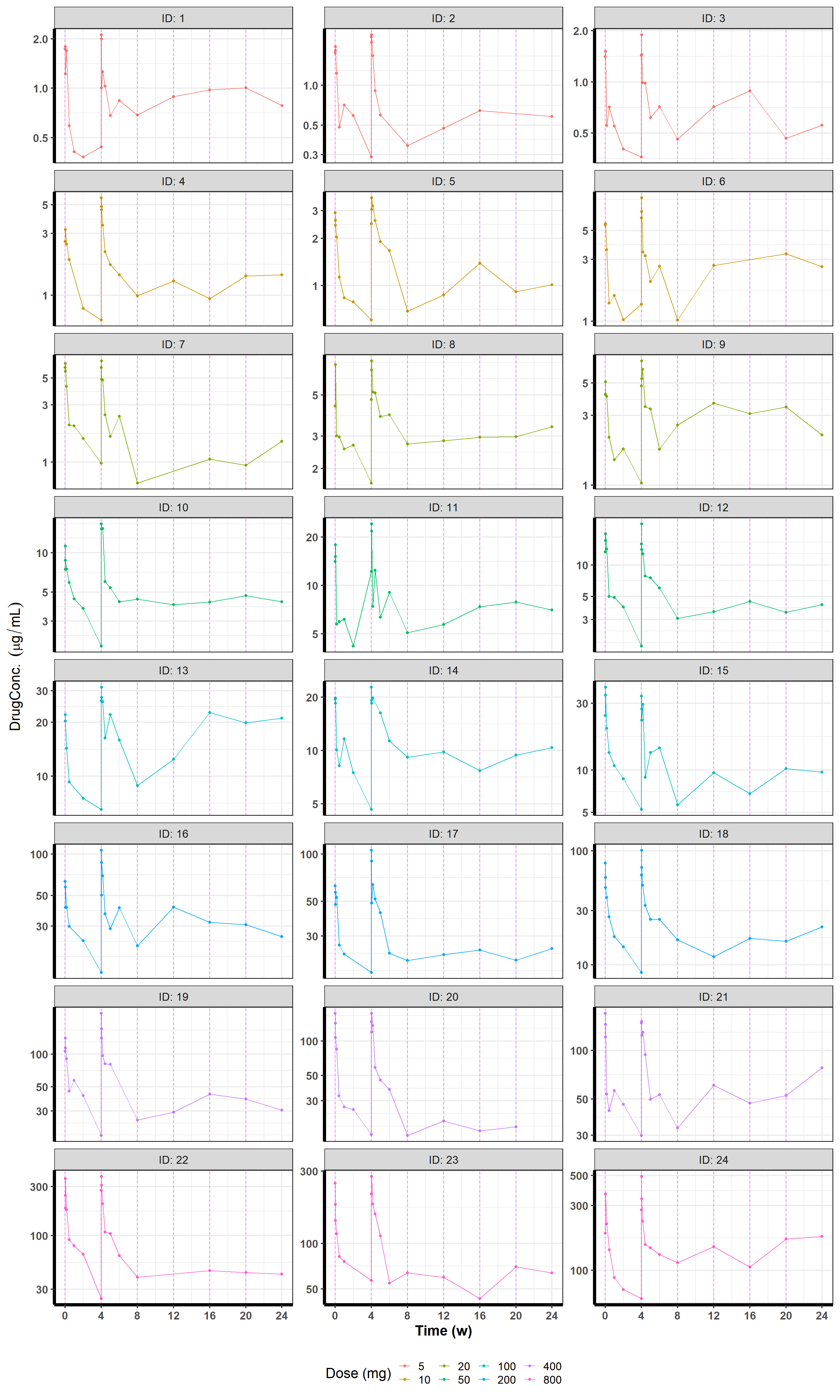
3.3.4 Eliciting Prior Information
The use of the prior distribution can range from being a nuisance that serves simply as a catalyst that allows us to express uncertainty via Bayes’ theorem to a means to stabilize the sampling algorithm to actually incorporating knowledge about the parameter(s) before collecting data. We will discuss a couple common methods for eliciting prior information and setting your prior distributions.
3.3.4.1 Drug Class and/or Historical Information
A simple method that I’ll show here is to look at other drugs in the same class. For this example I used “true” PK parameters that are similar to a monoclonal antibody (mAb) I’ve worked on in the past to simulate this data. Since this fictional drug is a mAb, I can look at this paper to see a review of published clearances and volumes of distribution for other mAbs:
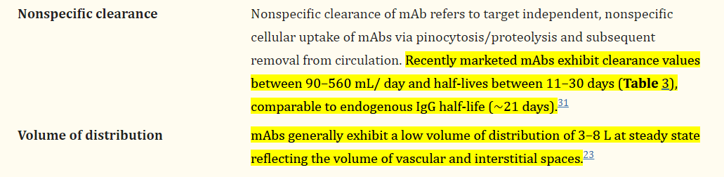
I will set my priors in such a way that there is plenty of prior mass over the values that we’ve previously seen in mAbs (in red) but not so wide that the sampler will go looking at non-sensical values like \(CL = 300 \frac{L}{d}\)
\[\begin{align} TVCL &\sim Half-Cauchy\;(0, \; 2) \notag \\ TVVC &\sim Half-Cauchy\;(0, \; 10) \end{align}\]
Code
my_length <- 200
dens_data <- tibble(parameter = rep(c("TVCL", "TVVC"), each = my_length),
value = c(seq(0, 10, length.out = my_length),
seq(0, 40, length.out = my_length))) %>%
bind_rows(tibble(parameter = rep(c("TVCL", "TVVC"), each = 2),
value = c(0.09, 0.56, 3, 8))) %>%
arrange(parameter, value) %>%
mutate(scale = if_else(parameter == "TVCL", 2, 10),
dens = dcauchy(value, scale = scale)/pcauchy(0, scale = scale))
p_cl <- ggplot(data = dens_data %>%
filter(parameter == "TVCL"),
aes(x = value, y = dens, group = parameter)) +
geom_line(size = 1.25) +
theme_bw(18) +
geom_area(mapping = aes(x = if_else(between(value, 0.09, 0.56), value, 0)),
fill = "red") +
scale_y_continuous(name = "Density",
limits = c(0, 0.34),
expand = c(0, 0)) +
scale_x_continuous(name = "Clearance (L/d)",
expand = c(0, 0),
breaks = seq(0, 10, by = 2.5),
labels = c("0", "2.5", "5", "7.5", "10"))
p_vc <- ggplot(data = dens_data %>%
filter(parameter == "TVVC"),
aes(x = value, y = dens, group = parameter)) +
geom_line(size = 1.25) +
theme_bw(18) +
geom_area(mapping = aes(x = if_else(between(value, 3, 8), value, 0)),
fill = "red") +
scale_y_continuous(name = "Density",
limits = c(0, 0.07),
expand = c(0, 0)) +
scale_x_continuous(name = "Volume (L)",
expand = c(0, 0))
p_cl | p_vc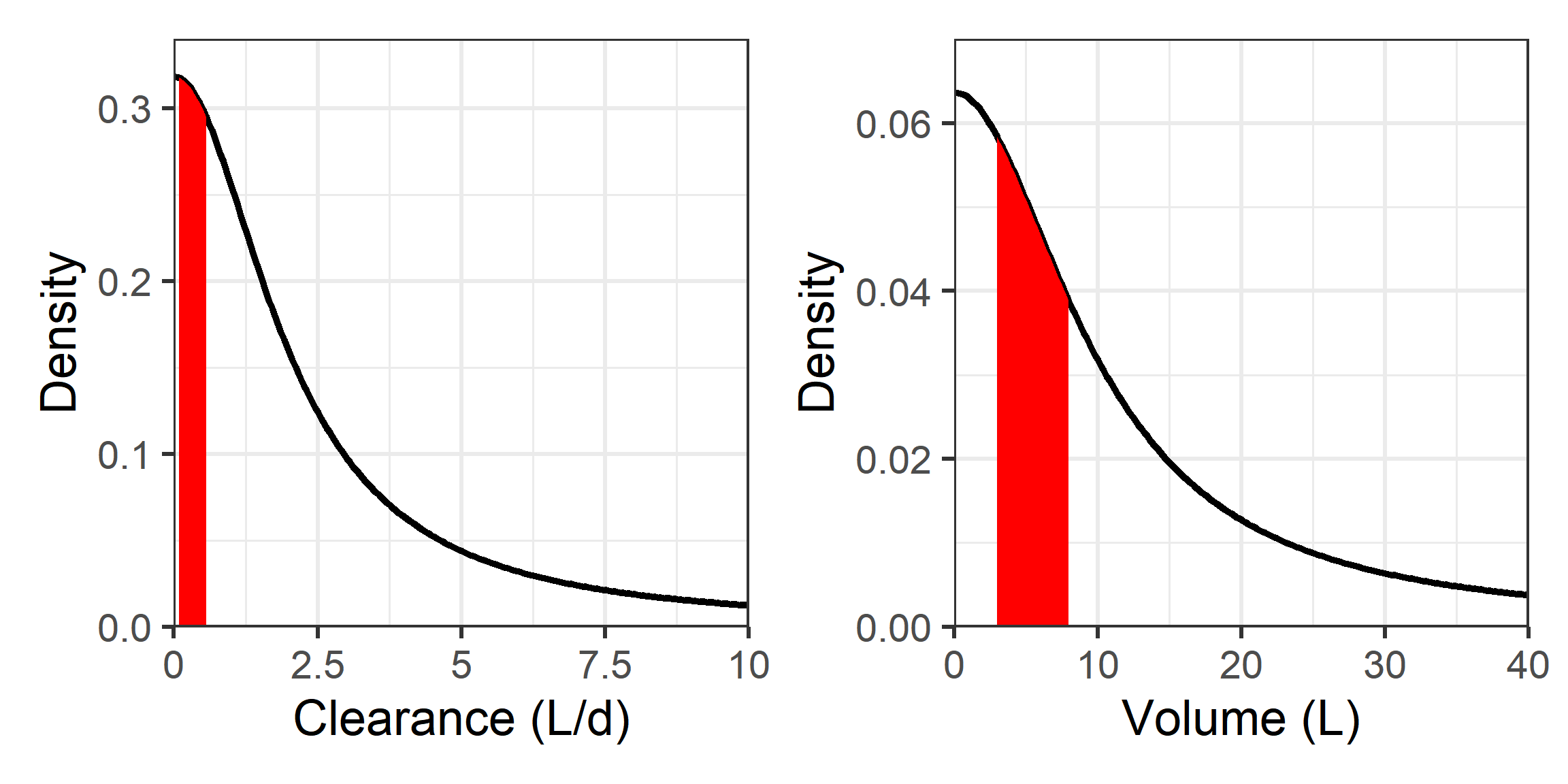
This could also be done with lognormal prior distributions (which might be a little more familiar in the PK/PD world):\[\begin{align} TVCL &\sim Lognormal\;(log(0.5), \; 1) \notag \\ TVVC &\sim Lognormal\;(log(6), \; 1) \end{align}\]
Code
dens_data_2 <- tibble(parameter = rep(c("TVCL", "TVVC"), each = my_length),
value = c(seq(0, 5, length.out = my_length),
seq(0, 40, length.out = my_length))) %>%
bind_rows(tibble(parameter = rep(c("TVCL", "TVVC"), each = 2),
value = c(0.09, 0.56, 3, 8))) %>%
arrange(parameter, value) %>%
mutate(location = if_else(parameter == "TVCL", log(0.5), log(6)),
scale = if_else(parameter == "TVCL", 1, 1),
dens = dlnorm(value, meanlog = location,
sdlog = scale))
p_cl_2 <- ggplot(data = dens_data_2 %>%
filter(parameter == "TVCL"),
aes(x = value, y = dens, group = parameter)) +
geom_line(size = 1.25) +
theme_bw(18) +
geom_area(mapping = aes(x = if_else(between(value, 0.09, 0.56), value, 0)),
fill = "red") +
scale_y_continuous(name = "Density",
limits = c(0, 1.35),
expand = c(0, 0)) +
scale_x_continuous(name = "Clearance (L/d)",
expand = c(0, 0),
breaks = seq(0, 5, by = 1),
labels = seq(0, 5, by = 1))
p_vc_2 <- ggplot(data = dens_data_2 %>%
filter(parameter == "TVVC"),
aes(x = value, y = dens, group = parameter)) +
geom_line(size = 1.25) +
theme_bw(18) +
geom_area(mapping = aes(x = if_else(between(value, 3, 8), value, 0)),
fill = "red") +
scale_y_continuous(name = "Density",
limits = c(0, 0.15),
expand = c(0, 0)) +
scale_x_continuous(name = "Volume (L)",
expand = c(0, 0))
p_cl_2 | p_vc_2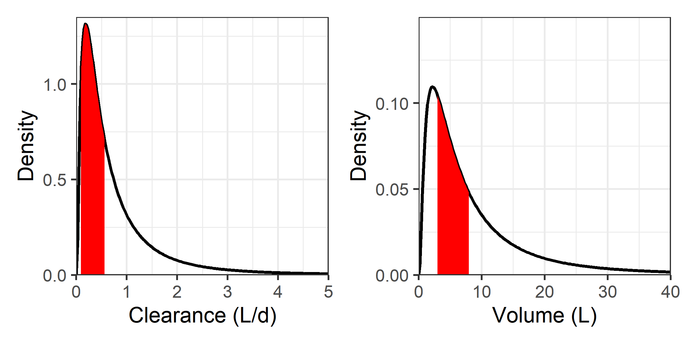
Either way, my goal here was to set a weakly informative prior by looking at historical estimates for drugs in the same class, then making sure there is plenty of prior mass over the range of previous estimates while also ruling out values that really wouldn’t make any sense. Then ideally the data will take it from there.
3.3.4.2 Priors for Nested Models and Occam’s Razor
Often times in pharmacometrics we extend our models because we believe they are failing to capture some aspect of the data. For example, extending a one compartment model to a two compartment model to account for two-phase elimination. Other examples in pharmacometrics abound such as delay compartments, nonlinear clearance, and exponential versus logistic tumor growth. These models are all nested in the sense that the less complex model is a special case of the more complex model with parameter values fixed to some constant. For example, a one compartment model can be thought of as a two compartment model where the \(Q\) parameter is fixed to zero, or in other words, a two compartment model with an infinitely informative prior with all of its mass on zero. At the other extreme is the extended model with completely uninformative priors on the additional parameters, which in practice can cause computational issues when data alone does not identify the additional parameters very well.
For nested models we can place priors on the extended parameters that give us the best of the both worlds. In a two compartment model for example, a Half-Cauchy prior on \(Q\) is a relaxation of the one compartment model that slightly favors the simpler explanation of \(Q=0\), but also allows for non-zero \(Q\) if the data provides enough evidence to support it. This idea of incorporating the principle of Occam’s razor in our inference via priors, relieves computational issues and is the principle behind modern complex non-parameteric models and tools like LASSO that can fit many parameters by regularizing to favor the simpler nested model.
3.3.4.3 Prior Predictive Checks
A wealth of prior information about the properties of our drugs exists in the form of published historical data, pre-clinical experiments, and basic physical constraints. However, for complex models we occasionally have parameters whose interpretation and relationship to data which we observe is unclear or highly complex. In these cases, prior predictive checks are a powerful tool for helping us elucidate these relationships and choose our priors. The principle is that while we may not always know reasonable values for a parameter in a complex model, we generally have a good understanding of reasonable values of our data. We briefly illustrate this using a two compartment model.
A prior predictive check simply consists of taking draws from your prior and simulating data using those draws. To do this, all we have to do is fit our model without any data. This can be done easily in Stan/Torsten by fitting a model as we normally would except we place the likelihood in an if-statement that controls whether we wants to draw from the prior only or the full posterior which includes both the prior and the likelihood. This is done in the two compartment model below where we use log-normal priors on the parameters.
Code
model_ppc <- cmdstan_model("Torsten/Fit/iv_2cmt_ppa_lognormal_priors_ppc.stan")
model_ppc$print()// IV Infusion
// Two-compartment PK Model
// IIV on CL, VC, Q, VP (full covariance matrix)
// proportional plus additive error - DV = CP(1 + eps_p) + eps_a
// Closed form solution using Torsten
// Implements threading for within-chain parallelization
functions{
array[] int sequence(int start, int end) {
array[end - start + 1] int seq;
for (n in 1:num_elements(seq)) {
seq[n] = n + start - 1;
}
return seq;
}
int num_between(int lb, int ub, array[] int y){
int n = 0;
for(i in 1:num_elements(y)){
if(y[i] >= lb && y[i] <= ub)
n = n + 1;
}
return n;
}
array[] int find_between(int lb, int ub, array[] int y) {
// vector[num_between(lb, ub, y)] result;
array[num_between(lb, ub, y)] int result;
int n = 1;
for (i in 1:num_elements(y)) {
if (y[i] >= lb && y[i] <= ub) {
result[n] = y[i];
n = n + 1;
}
}
return result;
}
vector find_between_vec(int lb, int ub, array[] int idx, vector y) {
vector[num_between(lb, ub, idx)] result;
int n = 1;
if(num_elements(idx) != num_elements(y)) reject("illegal input");
for (i in 1:rows(y)) {
if (idx[i] >= lb && idx[i] <= ub) {
result[n] = y[i];
n = n + 1;
}
}
return result;
}
real partial_sum_lpmf(array[] int seq_subj, int start, int end,
vector dv_obs, array[] int dv_obs_id, array[] int i_obs,
array[] real amt, array[] int cmt, array[] int evid,
array[] real time, array[] real rate, array[] real ii,
array[] int addl, array[] int ss,
array[] int subj_start, array[] int subj_end,
real TVCL, real TVVC, real TVQ, real TVVP,
vector omega, matrix L, matrix Z,
vector sigma, matrix L_Sigma,
int n_random, int n_subjects, int n_total){
real ptarget = 0;
row_vector[n_random] typical_values = to_row_vector({TVCL, TVVC, TVQ, TVVP});
matrix[n_subjects, n_random] eta = diag_pre_multiply(omega, L * Z)';
matrix[n_subjects, n_random] theta =
(rep_matrix(typical_values, n_subjects) .* exp(eta));
matrix[2, 2] R_Sigma = multiply_lower_tri_self_transpose(L_Sigma);
matrix[2, 2] Sigma = quad_form_diag(R_Sigma, sigma);
int N = end - start + 1; // number of subjects in this slice
vector[n_total] dv_ipred; // = rep_vector(0, n_total);
matrix[n_total, 3] x_ipred; // = rep_matrix(0, n_total, 2);
int n_obs_slice = num_between(subj_start[start], subj_end[end], i_obs);
array[n_obs_slice] int i_obs_slice = find_between(subj_start[start],
subj_end[end], i_obs);
vector[n_obs_slice] dv_obs_slice = find_between_vec(start, end,
dv_obs_id, dv_obs);
vector[n_obs_slice] ipred_slice;
for(n in 1:N){ // loop over subjects in this slice
int nn = n + start - 1; // nn is the ID of the current subject
row_vector[n_random] theta_nn = theta[nn]; // access the parameters for subject nn
real cl = theta_nn[1];
real vc = theta_nn[2];
real q = theta_nn[3];
real vp = theta_nn[4];
array[5] real theta_params = {cl, q, vc, vp, 0}; // The 0 is for KA. Skip the absorption
x_ipred[subj_start[nn]:subj_end[nn], ] =
pmx_solve_twocpt(time[subj_start[nn]:subj_end[nn]],
amt[subj_start[nn]:subj_end[nn]],
rate[subj_start[nn]:subj_end[nn]],
ii[subj_start[nn]:subj_end[nn]],
evid[subj_start[nn]:subj_end[nn]],
cmt[subj_start[nn]:subj_end[nn]],
addl[subj_start[nn]:subj_end[nn]],
ss[subj_start[nn]:subj_end[nn]],
theta_params)';
dv_ipred[subj_start[nn]:subj_end[nn]] =
x_ipred[subj_start[nn]:subj_end[nn], 2] ./ vc;
}
ipred_slice = dv_ipred[i_obs_slice];
ptarget += normal_lpdf(dv_obs_slice | ipred_slice,
sqrt(square(ipred_slice) * Sigma[1, 1] +
Sigma[2, 2] +
2 * ipred_slice * Sigma[2, 1]));
return ptarget;
}
}
data{
int n_subjects;
int n_total;
int n_obs;
array[n_obs] int i_obs;
array[n_total] int ID;
array[n_total] real amt;
array[n_total] int cmt;
array[n_total] int evid;
array[n_total] real rate;
array[n_total] real ii;
array[n_total] int addl;
array[n_total] int ss;
array[n_total] real time;
vector[n_total] dv;
array[n_subjects] int subj_start;
array[n_subjects] int subj_end;
real<lower = 0> location_tvcl; // Prior Location parameter for CL
real<lower = 0> location_tvvc; // Prior Location parameter for VC
real<lower = 0> location_tvq; // Prior Location parameter for Q
real<lower = 0> location_tvvp; // Prior Location parameter for VP
real<lower = 0> scale_tvcl; // Prior Scale parameter for CL
real<lower = 0> scale_tvvc; // Prior Scale parameter for VC
real<lower = 0> scale_tvq; // Prior Scale parameter for Q
real<lower = 0> scale_tvvp; // Prior Scale parameter for VP
real<lower = 0> scale_omega_cl; // Prior scale parameter for omega_cl
real<lower = 0> scale_omega_vc; // Prior scale parameter for omega_vc
real<lower = 0> scale_omega_q; // Prior scale parameter for omega_q
real<lower = 0> scale_omega_vp; // Prior scale parameter for omega_vp
real<lower = 0> lkj_df_omega; // Prior degrees of freedom for omega cor mat
real<lower = 0> scale_sigma_p; // Prior Scale parameter for proportional error
real<lower = 0> scale_sigma_a; // Prior Scale parameter for additive error
real<lower = 0> lkj_df_sigma; // Prior degrees of freedom for sigma cor mat
// If set to 1, don't include the likelihood so we can do prior predictive checks
int <lower = 0, upper = 1> prior_only;
}
transformed data{
int grainsize = 1;
vector[n_obs] dv_obs = dv[i_obs];
array[n_obs] int dv_obs_id = ID[i_obs];
int n_random = 4; // Number of random effects
array[n_random] real scale_omega = {scale_omega_cl, scale_omega_vc,
scale_omega_q, scale_omega_vp};
array[2] real scale_sigma = {scale_sigma_p, scale_sigma_a};
array[n_subjects] int seq_subj = sequence(1, n_subjects); // reduce_sum over subjects
}
parameters{
real<lower = 0> TVCL;
real<lower = 0> TVVC;
real<lower = 0> TVQ;
real<lower = 0> TVVP;
vector<lower = 0>[n_random] omega;
cholesky_factor_corr[n_random] L;
vector<lower = 0>[2] sigma;
cholesky_factor_corr[2] L_Sigma;
matrix[n_random, n_subjects] Z;
}
model{
// Priors
TVCL ~ lognormal(log(location_tvcl), scale_tvcl);
TVVC ~ lognormal(log(location_tvvc), scale_tvvc);
TVQ ~ lognormal(log(location_tvq), scale_tvq);
TVVP ~ lognormal(log(location_tvvp), scale_tvvp);
omega ~ normal(0, scale_omega);
L ~ lkj_corr_cholesky(lkj_df_omega);
sigma ~ normal(0, scale_sigma);
L_Sigma ~ lkj_corr_cholesky(lkj_df_sigma);
to_vector(Z) ~ std_normal();
// Likelihood
if(prior_only == 0) {
target += reduce_sum(partial_sum_lupmf, seq_subj, grainsize,
dv_obs, dv_obs_id, i_obs,
amt, cmt, evid, time,
rate, ii, addl, ss, subj_start, subj_end,
TVCL, TVVC, TVQ, TVVP, omega, L, Z,
sigma, L_Sigma,
n_random, n_subjects, n_total);
}
}
generated quantities{
real<lower = 0> sigma_p = sigma[1];
real<lower = 0> sigma_a = sigma[2];
real<lower = 0> sigma_sq_p = square(sigma_p);
real<lower = 0> sigma_sq_a = square(sigma_a);
real<lower = 0> omega_cl = omega[1];
real<lower = 0> omega_vc = omega[2];
real<lower = 0> omega_q = omega[3];
real<lower = 0> omega_vp = omega[4];
real<lower = 0> omega_sq_cl = square(omega_cl);
real<lower = 0> omega_sq_vc = square(omega_vc);
real<lower = 0> omega_sq_q = square(omega_q);
real<lower = 0> omega_sq_vp = square(omega_vp);
real cor_cl_vc;
real cor_cl_q;
real cor_cl_vp;
real cor_vc_q;
real cor_vc_vp;
real cor_q_vp;
real omega_cl_vc;
real omega_cl_q;
real omega_cl_vp;
real omega_vc_q;
real omega_vc_vp;
real omega_q_vp;
real cor_p_a;
real sigma_p_a;
vector[n_subjects] eta_cl;
vector[n_subjects] eta_vc;
vector[n_subjects] eta_q;
vector[n_subjects] eta_vp;
vector[n_subjects] CL;
vector[n_subjects] VC;
vector[n_subjects] Q;
vector[n_subjects] VP;
vector[n_obs] ipred;
vector[n_obs] pred;
vector[n_obs] dv_ppc;
vector[n_obs] log_lik;
vector[n_obs] res;
vector[n_obs] wres;
vector[n_obs] ires;
vector[n_obs] iwres;
{
row_vector[n_random] typical_values = to_row_vector({TVCL, TVVC, TVQ, TVVP});
matrix[n_random, n_random] R = multiply_lower_tri_self_transpose(L);
matrix[n_random, n_random] Omega = quad_form_diag(R, omega);
matrix[2, 2] R_Sigma = multiply_lower_tri_self_transpose(L_Sigma);
matrix[2, 2] Sigma = quad_form_diag(R_Sigma, sigma);
matrix[n_subjects, n_random] eta = diag_pre_multiply(omega, L * Z)';
matrix[n_subjects, n_random] theta =
(rep_matrix(typical_values, n_subjects) .* exp(eta));
vector[n_total] dv_pred;
matrix[n_total, 3] x_pred;
vector[n_total] dv_ipred;
matrix[n_total, 3] x_ipred;
array[5] real theta_params_tv = {TVCL, TVQ, TVVC, TVVP, 0}; // 0 is for KA to skip absorption
eta_cl = col(eta, 1);
eta_vc = col(eta, 2);
eta_q = col(eta, 3);
eta_vp = col(eta, 4);
CL = col(theta, 1);
VC = col(theta, 2);
Q = col(theta, 3);
VP = col(theta, 4);
cor_cl_vc = R[1, 2];
cor_cl_q = R[1, 3];
cor_cl_vp = R[1, 4];
cor_vc_q = R[2, 3];
cor_vc_vp = R[2, 4];
cor_q_vp = R[3, 4];
omega_cl_vc = Omega[1, 2];
omega_cl_q = Omega[1, 3];
omega_cl_vp = Omega[1, 4];
omega_vc_q = Omega[2, 3];
omega_vc_vp = Omega[2, 4];
omega_q_vp = Omega[3, 4];
cor_p_a = R_Sigma[2, 1];
sigma_p_a = Sigma[2, 1];
for(j in 1:n_subjects){
array[5] real theta_params = {CL[j], Q[j], VC[j], VP[j], 0};
x_ipred[subj_start[j]:subj_end[j],] =
pmx_solve_twocpt(time[subj_start[j]:subj_end[j]],
amt[subj_start[j]:subj_end[j]],
rate[subj_start[j]:subj_end[j]],
ii[subj_start[j]:subj_end[j]],
evid[subj_start[j]:subj_end[j]],
cmt[subj_start[j]:subj_end[j]],
addl[subj_start[j]:subj_end[j]],
ss[subj_start[j]:subj_end[j]],
theta_params)';
dv_ipred[subj_start[j]:subj_end[j]] =
x_ipred[subj_start[j]:subj_end[j], 2] ./ VC[j];
x_pred[subj_start[j]:subj_end[j],] =
pmx_solve_twocpt(time[subj_start[j]:subj_end[j]],
amt[subj_start[j]:subj_end[j]],
rate[subj_start[j]:subj_end[j]],
ii[subj_start[j]:subj_end[j]],
evid[subj_start[j]:subj_end[j]],
cmt[subj_start[j]:subj_end[j]],
addl[subj_start[j]:subj_end[j]],
ss[subj_start[j]:subj_end[j]],
theta_params_tv)';
dv_pred[subj_start[j]:subj_end[j]] =
x_pred[subj_start[j]:subj_end[j], 2] ./ TVVC;
}
pred = dv_pred[i_obs];
ipred = dv_ipred[i_obs];
}
res = dv_obs - pred;
ires = dv_obs - ipred;
for(i in 1:n_obs){
real ipred_tmp = ipred[i];
real sigma_tmp = sqrt(square(ipred_tmp) * sigma_sq_p + sigma_sq_a +
2*ipred_tmp*sigma_p_a);
dv_ppc[i] = normal_rng(ipred_tmp, sigma_tmp);
log_lik[i] = normal_lpdf(dv_obs[i] | ipred_tmp, sigma_tmp);
wres[i] = res[i]/sigma_tmp;
iwres[i] = ires[i]/sigma_tmp;
}
}We prepare the data as we normally would for Stan/Torsten except we include a new toggle prior_only and set it to 1. This data preparation step is mostly just book keeping to tell Stan and Torsten how many patients we’re fitting, how many observations, and the indices of each patient in the data frame we’re passing in.
We also specify the priors in this data preparation step. We start with the log-normal priors specified above along with vague log-normal priors on the second compartment volume and transfer rate.
The goal is to see whether for the prior values considered, the data generated from those priors, in this case PK concentration over time, results in sensible values and values that are able to capture your data. As an aside, priors can be thought to set the prior values considered in our search space where we will try to find all the combinations of parameters that reasonably fit our data. From this perspective it is easy to see why vague or no priors can lead to computational issues when data is not adequate, because you can be consdering an unbounded search space!
In general, you can start with vague priors and gradually tighten them so that your prior does not consider nonsensical values, e.g. values of concentration that are unreasonably high or low. Alternatively, you can start with highly informative priors centered around a value of the parameters where you know the solution makes sense, and you can gradually loosen them until the corresponding data generated from those priors considers all reasonable values of data you expect to see. We illustrate by starting somewhere in the middle, but the latter technique is sometimes preferred in practice as it is more computationally stable.
Code
nonmem_data <- read_csv("Data/iv_2cmt_no_bloq.csv",
na = ".") %>%
rename_all(tolower) %>%
rename(ID = "id",
DV = "dv") %>%
mutate(DV = if_else(is.na(DV), 5555555, DV)) # This value can be anything except NA. It'll be indexed away
n_subjects <- nonmem_data %>% # number of individuals
distinct(ID) %>%
count() %>%
deframe()
n_total <- nrow(nonmem_data) # total number of records
i_obs <- nonmem_data %>% # index for observation records
mutate(row_num = 1:n()) %>%
filter(evid == 0) %>%
select(row_num) %>%
deframe()
n_obs <- length(i_obs) # number of observation records
subj_start <- nonmem_data %>%
mutate(row_num = 1:n()) %>%
group_by(ID) %>%
slice_head(n = 1) %>%
ungroup() %>%
select(row_num) %>%
deframe()
subj_end <- c(subj_start[-1] - 1, n_total)
stan_data <- list(n_subjects = n_subjects,
n_total = n_total,
n_obs = n_obs,
i_obs = i_obs,
ID = nonmem_data$ID,
amt = nonmem_data$amt,
cmt = nonmem_data$cmt,
evid = nonmem_data$evid,
rate = nonmem_data$rate,
ii = nonmem_data$ii,
addl = nonmem_data$addl,
ss = nonmem_data$ss,
time = nonmem_data$time,
dv = nonmem_data$DV,
subj_start = subj_start,
subj_end = subj_end,
location_tvcl = 0.5, scale_tvcl = 1,
location_tvvc = 6, scale_tvvc = 1,
location_tvq = 1, scale_tvq = 2,
location_tvvp = 3, scale_tvvp = 2,
scale_omega_cl = 0.4,
scale_omega_vc = 0.4,
scale_omega_q = 0.4,
scale_omega_vp = 0.4,
lkj_df_omega = 2,
scale_sigma_p = 0.5,
scale_sigma_a = 1,
lkj_df_sigma = 2,
prior_only = 1L)After setting up the input data and our priors, we now fit the model as we normally would:
Code
fit_ppc1 <- model_ppc$sample(data = stan_data,
seed = 112358,
chains = 4,
parallel_chains = 4,
iter_warmup = 500,
iter_sampling = 1000,
adapt_delta = 0.8,
refresh = 500,
max_treedepth = 10,
init = function() list(TVCL = rlnorm(1, log(0.3), 0.3),
TVVC = rlnorm(1, log(6), 0.3),
TVQ = rlnorm(1, log(1), 0.3),
TVVP = rlnorm(1, log(3), 0.3),
omega = rlnorm(5, log(0.3), 0.3),
sigma = rlnorm(2, log(0.5), 0.3)))Running MCMC with 4 parallel chains...
Chain 1 Iteration: 1 / 1500 [ 0%] (Warmup)
Chain 2 Iteration: 1 / 1500 [ 0%] (Warmup)
Chain 3 Iteration: 1 / 1500 [ 0%] (Warmup)
Chain 4 Iteration: 1 / 1500 [ 0%] (Warmup)
Chain 1 Iteration: 500 / 1500 [ 33%] (Warmup)
Chain 1 Iteration: 501 / 1500 [ 33%] (Sampling)
Chain 2 Iteration: 500 / 1500 [ 33%] (Warmup)
Chain 2 Iteration: 501 / 1500 [ 33%] (Sampling)
Chain 3 Iteration: 500 / 1500 [ 33%] (Warmup)
Chain 3 Iteration: 501 / 1500 [ 33%] (Sampling)
Chain 4 Iteration: 500 / 1500 [ 33%] (Warmup)
Chain 4 Iteration: 501 / 1500 [ 33%] (Sampling)
Chain 2 Iteration: 1000 / 1500 [ 66%] (Sampling)
Chain 1 Iteration: 1000 / 1500 [ 66%] (Sampling)
Chain 4 Iteration: 1000 / 1500 [ 66%] (Sampling)
Chain 3 Iteration: 1000 / 1500 [ 66%] (Sampling)
Chain 1 Iteration: 1500 / 1500 [100%] (Sampling)
Chain 4 Iteration: 1500 / 1500 [100%] (Sampling)
Chain 2 Iteration: 1500 / 1500 [100%] (Sampling)
Chain 3 Iteration: 1500 / 1500 [100%] (Sampling)
Chain 1 finished in 24.4 seconds.
Chain 2 finished in 24.5 seconds.
Chain 4 finished in 24.4 seconds.
Chain 3 finished in 24.5 seconds.
All 4 chains finished successfully.
Mean chain execution time: 24.5 seconds.
Total execution time: 25.1 seconds.We now plot the concentration data generated from our use of priors. Specifically, we look at concentration values at the first few study time points using the dosing regimen that was given to the first three patients in our study. The concentration values are generated in Stan’s generated quantities block by solving the two compartment model at the various values drawn from our prior. No additional observational noise is added (although we could if we wanted to also tune the prior on \(\sigma\)). We summarize the drawn concentration samples with medians along with 5% and 95% quantiles. Lastly, we overlay the actual data of our three patients who actually were assigned this dosing regimen over these prior predictive samples to give us additional perspective on whether the simulated concentration values generated from our prior are reasonable.
Code
ipred_ppc <- fit_ppc1$summary("ipred") %>%
bind_cols(filter(nonmem_data, evid == 0)) %>%
filter(ID == 1, time <= 28)
nonmem_data_patient123 <-nonmem_data %>%
filter(evid == 0) %>%
mutate(i = row_number()) %>%
filter(ID %in% c(1, 2, 3), time <= 28)
ipred_ppc %>%
ggplot(aes(time, median)) +
geom_pointrange(aes(ymin = q5, ymax = q95)) +
geom_point(aes(time, DV), color = "red", data = nonmem_data_patient123) +
scale_y_log10() +
theme_bw(20) +
scale_x_continuous(name = "Time (d)") +
scale_y_log10(name = "Drug Concentration (ug/mL)")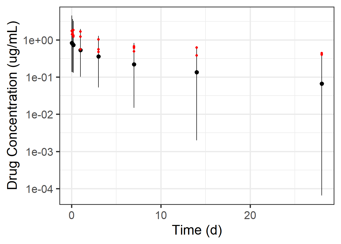
From the plot it seems like we are considering a reasonable range of solutions for early values of concentration with our prior. However, for the later value, just before the second dose, we are clearly considering values that are unreasonably low. We know that for a mAB with a long half-life we should not have such low concentration after 28 days. Furthermore none of our observed data comes close to being that low. To explore further which parameter values that we are considering with our prior correspond to these unreasonable values, we can plot a scatter plot of our prior samples versus the simulated value at this time point (called ipred[6] in our model).
Code
mcmc_pairs(fit_ppc1$draws(c("TVCL", "TVVC", "TVQ", "TVVP", "ipred[6]")),
diag_fun = "dens",
transformations = "log")
We can see that the particularly low values of ipred[6] correspond closely to high TVCL, low TVVC, and somewhat to low TVVP. We can thus limit our priors in these areas to give less weight to these values. Note that the most extreme points of ipred[6] occur when both TVCL is large and TVVC is small. This could suggest that we want a prior on these parameters with a negative correlation, although we’ll keep the priors uncorrelated for now. For the sake of the example, we’re assuming we don’t have much intuition about the parameters but we know that the posterior of volume and clearance are often negatively correlated.
Code
stan_data2 <- stan_data
stan_data2$location_tvcl <- 0.2
stan_data2$scale_tvcl <- 0.5
stan_data2$location_tvvc <- 5
stan_data2$scale_tvvc <- 0.5
stan_data2$scale_tvvp <- 1Code
fit_ppc2 <- model_ppc$sample(data = stan_data2,
seed = 112358,
chains = 4,
parallel_chains = 4,
iter_warmup = 500,
iter_sampling = 1000,
adapt_delta = 0.8,
refresh = 500,
max_treedepth = 10,
init = function() list(TVCL = rlnorm(1, log(0.3), 0.3),
TVVC = rlnorm(1, log(6), 0.3),
TVQ = rlnorm(1, log(1), 0.3),
TVVP = rlnorm(1, log(3), 0.3),
omega = rlnorm(5, log(0.3), 0.3),
sigma = rlnorm(2, log(0.5), 0.3)))Running MCMC with 4 parallel chains...
Chain 1 Iteration: 1 / 1500 [ 0%] (Warmup)
Chain 2 Iteration: 1 / 1500 [ 0%] (Warmup)
Chain 3 Iteration: 1 / 1500 [ 0%] (Warmup)
Chain 4 Iteration: 1 / 1500 [ 0%] (Warmup)
Chain 1 Iteration: 500 / 1500 [ 33%] (Warmup)
Chain 1 Iteration: 501 / 1500 [ 33%] (Sampling)
Chain 2 Iteration: 500 / 1500 [ 33%] (Warmup)
Chain 2 Iteration: 501 / 1500 [ 33%] (Sampling)
Chain 3 Iteration: 500 / 1500 [ 33%] (Warmup)
Chain 3 Iteration: 501 / 1500 [ 33%] (Sampling)
Chain 4 Iteration: 500 / 1500 [ 33%] (Warmup)
Chain 4 Iteration: 501 / 1500 [ 33%] (Sampling)
Chain 1 Iteration: 1000 / 1500 [ 66%] (Sampling)
Chain 4 Iteration: 1000 / 1500 [ 66%] (Sampling)
Chain 2 Iteration: 1000 / 1500 [ 66%] (Sampling)
Chain 3 Iteration: 1000 / 1500 [ 66%] (Sampling)
Chain 1 Iteration: 1500 / 1500 [100%] (Sampling)
Chain 4 Iteration: 1500 / 1500 [100%] (Sampling)
Chain 2 Iteration: 1500 / 1500 [100%] (Sampling)
Chain 1 finished in 23.9 seconds.
Chain 3 Iteration: 1500 / 1500 [100%] (Sampling)
Chain 4 finished in 23.9 seconds.
Chain 2 finished in 24.1 seconds.
Chain 3 finished in 24.2 seconds.
All 4 chains finished successfully.
Mean chain execution time: 24.0 seconds.
Total execution time: 24.6 seconds.Code
ipred_ppc <- fit_ppc2$summary("ipred") %>%
bind_cols(filter(nonmem_data, evid == 0)) %>%
filter(ID == 1, time <= 28)
ipred_ppc %>%
ggplot(aes(time, median)) +
geom_pointrange(aes(ymin = q5, ymax = q95)) +
geom_point(aes(time, DV), color = "red", data = nonmem_data_patient123) +
scale_y_log10() +
theme_bw(20) +
scale_x_continuous(name = "Time (d)") +
scale_y_log10(name = "Drug Concentration (ug/mL)")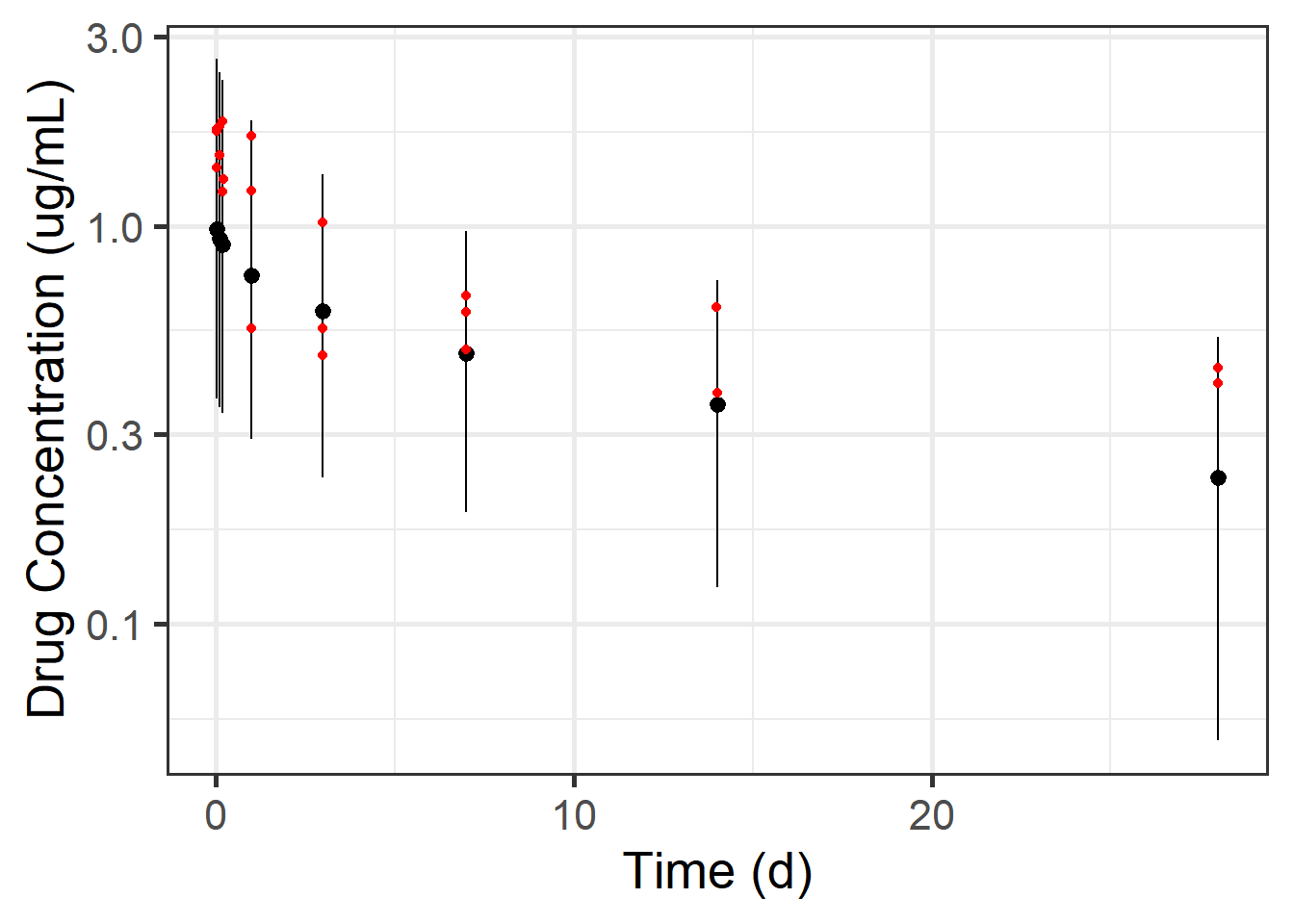
Now with our remodel refit to give us our new prior predictive check with the adjusted priors we can see that for ipred[6] we are no longer considering unreasonably low values. Meanwhile at the other time point we consider a reasonable range of parameter values that lead to concentrations which encompass our observed data. Further tuning could be done to broaden or tighten the search space as desired.
As a final and related note to this section, we briefly mention the concept of placing priors directly on derived quantities. In our prior predictive check example we knew reasonable ranges for our concentration (data) values, but we didn’t know reasonable values for our parameters or how they relate to the resulting concentrations. We thus hand-tuned our priors so that the resulting prior parameter values considered corresponded to reasonable output concentration solutions. In Stan there is indeed an even more direct way to do this. We can place priors on parameter-derived quantities directly! For example, we can place a lognormal prior on ipred[6] directly in our Stan model block so that unreasonably low values are avoided. Since ipred[6] is of course a function of the parameters, this induces a prior on the parameters.
Stan allows a lot of creativity on priors on derived quantities, as long as it’s expressible in an equation. For example we can specify a lognormal in the resulting amount (instead of concentration) of drug at a particular time point and specify that we think it should be no less than 1 10,000th of the dose after an hour. We can also place priors on things like half life for which we know the expression of as a function of parameters (incidentally this will induce a prior on volume and clearance that has a negative correlation).
3.3.4.4 Flat and Other “non-informative” Priors
People often try to be as “objective” as possible, so they use either a flat prior or an extremely wide prior. For example, in the NONMEM Users Guide, they use a multivariate normal prior distribution on the (log-)population parameters:
\[\begin{align} \begin{pmatrix} log(TVCL) \\ log(TVVC) \\ log(TVQ) \\ log(TVVP) \\ log(TVKA) \\ \end{pmatrix} \sim Normal\left( \begin{pmatrix} 2 \\ 2 \\ 2 \\ 2 \\ 2 \\ \end{pmatrix} , \; \begin{pmatrix} 10,000 & 0 & 0 & 0 & 0 \\ 0 & 10,000 & 0 & 0 & 0 \\ 0 & 0 & 10,000 & 0 & 0 \\ 0 & 0 & 0 & 10,000 & 0 \\ 0 & 0 & 0 & 0 & 10,000 \\ \end{pmatrix} \right) \notag \\ \end{align}\]and say “because variances are very large, this means that the prior information on THETAS is highly uninformative.” However, if we look at this distribution after transforming to the natural space (i.e. \(TVVC = exp(log(TVVC))\)), then we see that this distribution is not at all uninformative:
Code
data_uninformative <- tibble(TVVC = c(seq(0, 15, by = 0.0001), seq(16, 100,
by = 1),
seq(101, 10001, by = 10))) %>%
mutate(dens = dlnorm(TVVC, log(2), sqrt(10000)))
p_non_informative <- ggplot(data_uninformative, aes(x = TVVC, y = dens)) +
geom_line() +
scale_x_continuous(limits = c(0, 100),
trans = "identity") +
scale_y_continuous(name = "Density",
trans = "identity") +
geom_hline(yintercept = 0) +
theme_bw(18) +
ggtitle('"Uninformative" Prior') +
theme(plot.title = element_text(hjust = 0.5))
plotly::ggplotly(p_non_informative)