Logistic Regression Hands-On With Solution

Load Relevant Libraries

library(summarytools)
library(tidyverse) 
library(brms)
library(bayesplot)
library(tidybayes) 
library(gridExtra) 
library(patchwork) 

A simulated dataset for this exercise simlrcovs.csv was developed. It has the following columns:

1. DOSE: Dose of drug in mg [20, 50, 100, 200 mg]
2. CAVG: Average concentration until the time of the event (mg/L)
3. ECOG: ECOG performance status [0 = Fully active; 1 = Restricted in physical activity]
4. RACE: Race [1 = Others; 2 = White]
5. SEX: Sex [1 = Female; 2 = Male]
6. BRNMETS: Brain metastasis [1 = Yes; 0 = No]
7. DV: Event [1 = Yes; 0 = No]

Import Dataset

# Read the dataset
hoRaw <- read.csv("data/simlrcovs.csv") %>% 
  as_tibble()

Data Processing

Convert categorical explanatory variables to factors

hoData <- hoRaw %>% 
  mutate(ECOG = factor(ECOG, levels = c(0, 1), labels = c("Active", "Restricted")),
         RACE = factor(RACE, levels = c(0, 1), labels = c("White", "Others")),
         SEX = factor(SEX, levels = c(0, 1), labels = c("Male", "Female")),
         BRNMETS = factor(BRNMETS, levels = c(0, 1), labels = c("No", "Yes")))
hoData

# A tibble: 200 x 7
    DOSE  CAVG ECOG       RACE   SEX    BRNMETS    DV
   <int> <dbl> <fct>      <fct>  <fct>  <fct>   <int>
 1    20  203. Active     White  Female Yes         0
 2    20  202. Restricted White  Female No          0
 3    20  287. Restricted Others Female No          0
 4    20  174. Restricted Others Male   Yes         0
 5    20  270. Active     Others Male   Yes         0
 6    20  265. Active     Others Female No          1
 7    20  206. Restricted Others Female No          0
 8    20  253. Active     Others Male   No          1
 9    20  186. Active     White  Male   No          0
10    20  186. Restricted Others Female No          1
# ... with 190 more rows

Data Summary

print(summarytools::dfSummary(hoData,
          varnumbers = FALSE,
          valid.col = FALSE,
          graph.magnif = 0.76),
      method = "render")

Data Frame Summary

hoData
Dimensions: 200 x 7
Duplicates: 0

Variable	Stats / Values	Freqs (% of Valid)	Graph	Missing
DOSE [integer]	Mean (sd) : 92.5 (68.5) min ≤ med ≤ max: 20 ≤ 75 ≤ 200 IQR (CV) : 82.5 (0.7)	20 : 50 ( 25.0% ) 50 : 50 ( 25.0% ) 100 : 50 ( 25.0% ) 200 : 50 ( 25.0% )		0 (0.0%)
CAVG [numeric]	Mean (sd) : 1155.1 (918.3) min ≤ med ≤ max: 164 ≤ 928.6 ≤ 3791.7 IQR (CV) : 1423.5 (0.8)	200 distinct values		0 (0.0%)
ECOG [factor]	1. Active 2. Restricted	122 ( 61.0% ) 78 ( 39.0% )		0 (0.0%)
RACE [factor]	1. White 2. Others	70 ( 35.0% ) 130 ( 65.0% )		0 (0.0%)
SEX [factor]	1. Male 2. Female	90 ( 45.0% ) 110 ( 55.0% )		0 (0.0%)
BRNMETS [factor]	1. No 2. Yes	145 ( 72.5% ) 55 ( 27.5% )		0 (0.0%)
DV [integer]	Min : 0 Mean : 0.5 Max : 1	0 : 95 ( 47.5% ) 1 : 105 ( 52.5% )		0 (0.0%)

Model Fit

With all covariates except DOSE (since we have exposure as a driver)

hofit1 <-  brm(DV ~ CAVG + ECOG + RACE + SEX + BRNMETS,
           data = hoData,
           family = bernoulli(),
           chains = 4,
           warmup = 1000,
           iter = 2000,
           seed = 12345,
           refresh = 0,
           backend = "cmdstanr")
# freqhofit <-  glm(DV ~ CAVG + ECOG + RACE + SEX + BRNMETS,
#                family = "binomial",
#                data = hoData)
# summary(freqhofit)

Model Evaluation

summary(hofit1)

 Family: bernoulli 
  Links: mu = logit 
Formula: DV ~ CAVG + ECOG + RACE + SEX + BRNMETS 
   Data: hoData (Number of observations: 200) 
  Draws: 4 chains, each with iter = 2000; warmup = 1000; thin = 1;
         total post-warmup draws = 4000

Population-Level Effects: 
               Estimate Est.Error l-95% CI u-95% CI Rhat Bulk_ESS Tail_ESS
Intercept         -1.67      0.44    -2.56    -0.84 1.00     4103     3331
CAVG               0.00      0.00     0.00     0.00 1.00     4075     2528
ECOGRestricted    -0.47      0.34    -1.14     0.20 1.00     3892     2734
RACEOthers         1.45      0.36     0.76     2.18 1.00     3795     2389
SEXFemale         -0.21      0.32    -0.84     0.41 1.00     3662     2737
BRNMETSYes         0.20      0.37    -0.51     0.93 1.00     4029     2623

Draws were sampled using sample(hmc). For each parameter, Bulk_ESS
and Tail_ESS are effective sample size measures, and Rhat is the potential
scale reduction factor on split chains (at convergence, Rhat = 1).

fixef(hofit1)

                    Estimate    Est.Error         Q2.5        Q97.5
Intercept      -1.6728321010 0.4356726064 -2.557614750 -0.840452675
CAVG            0.0009840576 0.0002037094  0.000591061  0.001394632
ECOGRestricted -0.4703165395 0.3379044752 -1.136986750  0.199271800
RACEOthers      1.4457574770 0.3599390856  0.756435900  2.179535750
SEXFemale      -0.2140195943 0.3187733320 -0.840274025  0.406492000
BRNMETSYes      0.2011028320 0.3668881875 -0.506824900  0.928938150

Final Model

hofit2 <-  brm(DV ~ CAVG + RACE,
           data = hoData,
           family = bernoulli(),
           chains = 4,
           warmup = 1000,
           iter = 2000,
           seed = 12345,
           refresh = 0,
           backend = "cmdstanr")

Summary

summary(hofit2)

 Family: bernoulli 
  Links: mu = logit 
Formula: DV ~ CAVG + RACE 
   Data: hoData (Number of observations: 200) 
  Draws: 4 chains, each with iter = 2000; warmup = 1000; thin = 1;
         total post-warmup draws = 4000

Population-Level Effects: 
           Estimate Est.Error l-95% CI u-95% CI Rhat Bulk_ESS Tail_ESS
Intercept     -1.81      0.37    -2.55    -1.10 1.00     1962     2405
CAVG           0.00      0.00     0.00     0.00 1.00     4324     3163
RACEOthers     1.33      0.33     0.67     2.02 1.00     1732     1299

Draws were sampled using sample(hmc). For each parameter, Bulk_ESS
and Tail_ESS are effective sample size measures, and Rhat is the potential
scale reduction factor on split chains (at convergence, Rhat = 1).

fixef(hofit2)

                Estimate    Est.Error          Q2.5        Q97.5
Intercept  -1.8104092685 0.3672660010 -2.5532470000 -1.095532250
CAVG        0.0009570336 0.0002078047  0.0005667638  0.001378035
RACEOthers  1.3294440837 0.3334109622  0.6721790500  2.015080000

Model Convergence

hopost <- as_draws_df(hofit2, add_chain = T)
mcmc_trace(hopost[, -4],
           facet_args = list(ncol = 2)) +
  theme_bw()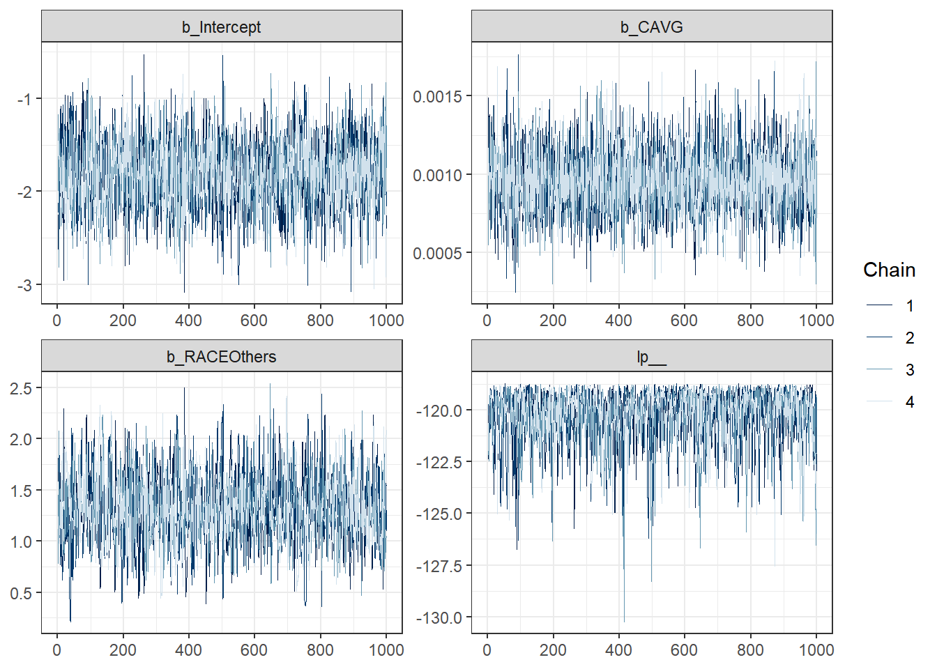

mcmc_acf(hopost[, -4]) + 
  theme_bw()

Visual Interpretation of the Model (Bonus Points!)

We can do this two ways.

Generate Posterior Probabilities Manually

Generate posterior probability of the event using the estimates and their associated posterior distributions

out <- hofit2 %>%
  spread_draws(b_Intercept, b_CAVG, b_RACEOthers) %>% 
  mutate(CAVG = list(seq(100, 4000, 10))) %>% 
  unnest(cols = c(CAVG)) %>%
  mutate(RACE = list(0:1)) %>% 
  unnest(cols = c(RACE)) %>% 
  mutate(PRED = exp(b_Intercept + b_CAVG * CAVG + b_RACEOthers * RACE)/(1 + exp(b_Intercept + b_CAVG * CAVG + b_RACEOthers * RACE))) %>%
  group_by(CAVG, RACE) %>%
  summarise(pred_m = mean(PRED, na.rm = TRUE),
            pred_low = quantile(PRED, prob = 0.025),
            pred_high = quantile(PRED, prob = 0.975)) %>% 
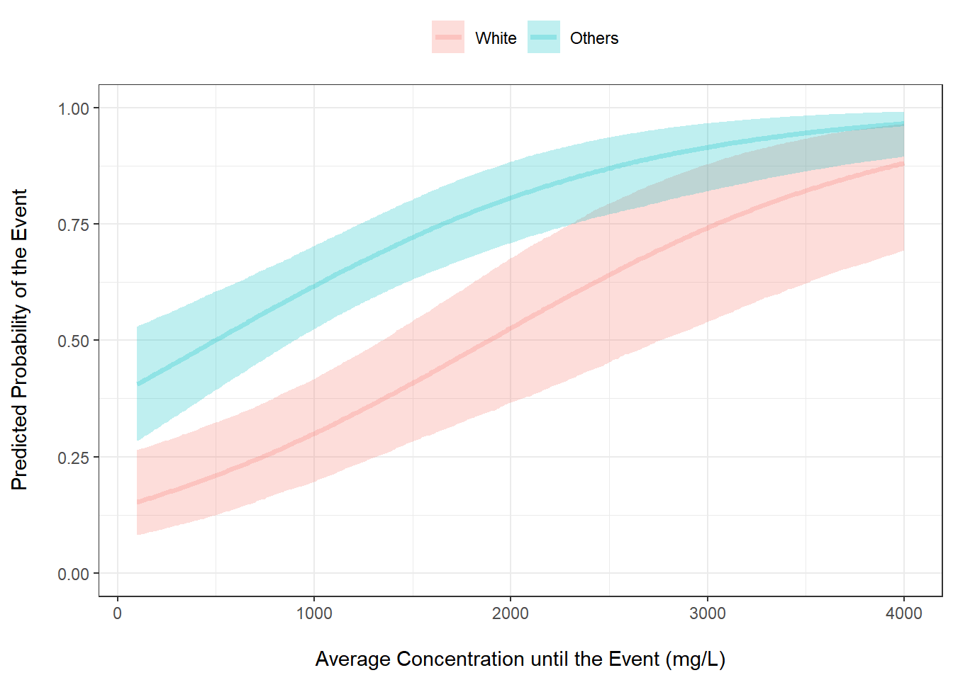
  mutate(RACE = factor(RACE, levels = c(0, 1), labels = c("White", "Others")))

Plot The Probability of the Event vs Average Concentration

out %>%
  ggplot(aes(x = CAVG, y = pred_m, color = factor(RACE))) +
  geom_line() +
  geom_ribbon(aes(ymin = pred_low, ymax = pred_high, fill = factor(RACE)), alpha = 0.2) +
  ylab("Predicted Probability of the Event\n") +
  xlab("\nAverage Concentration until the Event (mg/L)") +
  theme_bw() + 
  scale_fill_discrete("") +
  scale_color_discrete("") +
  theme(legend.position = "top")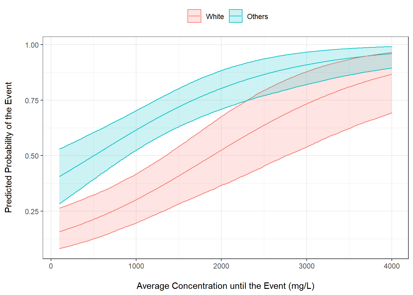

Generate Posterior Probabilities Using Helper Functions from brms and tidybayes

Generate posterior probability of the event using the estimates and their associated posterior distributions

out2 <- hofit2 %>%
  epred_draws(newdata = expand_grid(CAVG = seq(100, 4000, by = 10), 
                                    RACE = c("White", "Others")),
              value = "PRED") %>% 
  ungroup() %>% 
  mutate(RACE = factor(RACE, levels = c("White", "Others"), 
                       labels = c("White", "Others")))

Plot The Probability of the Event vs Average Concentration

out2 %>% 
  ggplot() +
  stat_lineribbon(aes(x = CAVG, y = PRED, color = RACE, fill = RACE), 
                  .width = 0.95, alpha = 0.25) +
  ylab("Predicted Probability of the Event\n") +
  xlab("\nAverage Concentration until the Event (mg/L)") +
  theme_bw() + 
  scale_fill_discrete("") +
  scale_color_discrete("") +
  theme(legend.position = "top") +
  ylim(c(0, 1))