Code
library(cmdstanr)
library(tidyverse)library(cmdstanr)
library(tidyverse)We’ll illustrate the basic components of a Stan program with a simple linear regression - the model is easy to understand so understanding the model doesn’t get in the way of learning basics of Stan code.
I’ll start out as simply as possible and then add tips and elements that can be carried over to other models.
Much of what is on this page isn’t necessarily a best practice. In fact, I wouldn’t write this model in raw Stan at all. I’d use rstanarm or brms - they both provide a ton of functionality that takes unnecessary extra effort to do in raw Stan. But I’ll write this in Stan in such a way as to highlight certain aspects of a Stan program and give tips that can be carried over to other models.
First we’ll create some data of the form \[ y_i = \alpha + \beta x_i + \epsilon_i, \;\;\;\;\;i = 1, \ldots, n, \]
and we’ll use true values \(\alpha = 2\), \(\beta = 3\), and \(\sigma = 6\).
set.seed(4384836)

n <- 30

alpha <- 2
beta <- 3
sigma <- 6

data <- tibble(x = runif(n, 20, 30)) %>%
  mutate(y = rnorm(n(), alpha + beta*x, sigma))

data %>%
  ggplot(aes(x = x, y = y)) +
  geom_point()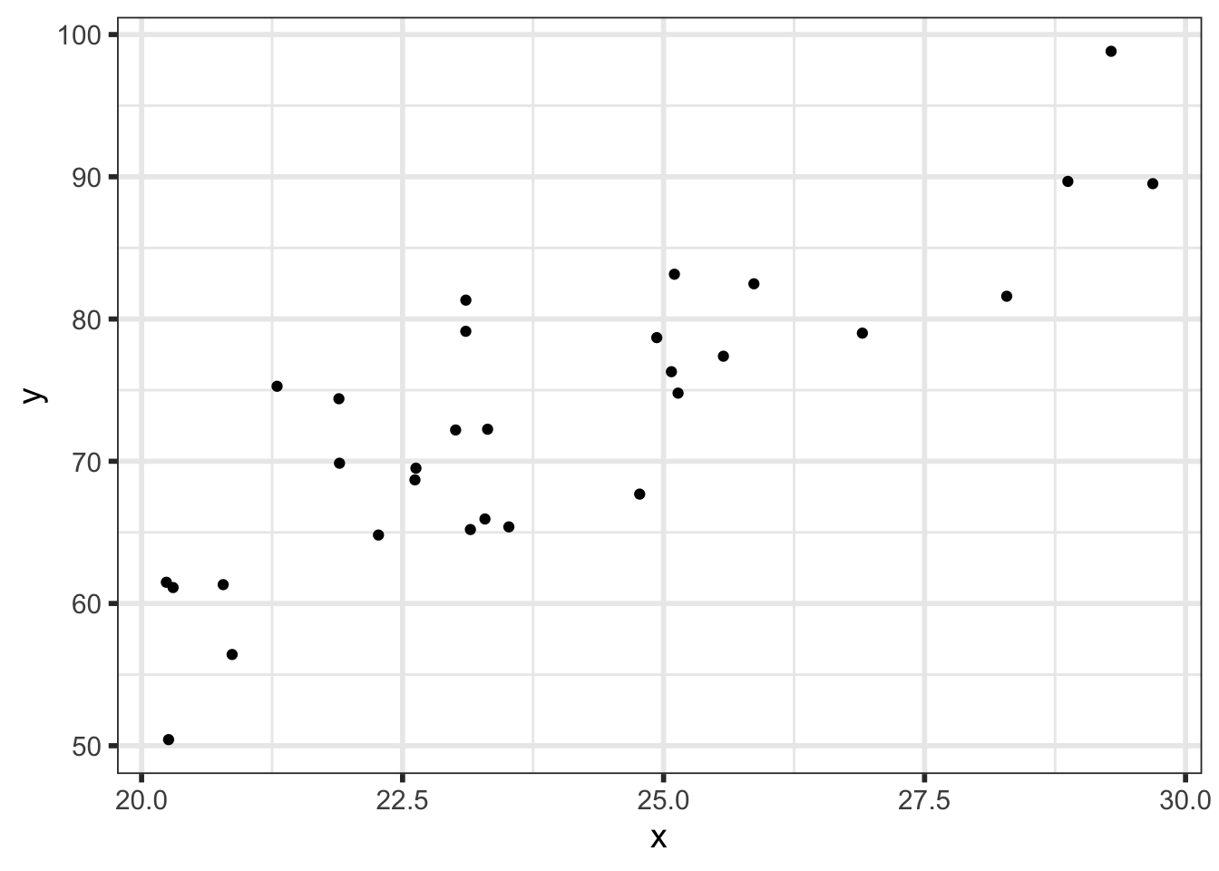
First, we will write out the model as simply as possible with no frills. Don’t write it this way in practice - use some of the tips shown later on this page.
We’ll write down the full statistical model:
\[ \begin{align} Y_i \; | \; \alpha, \beta, \sigma &\sim Normal(\alpha + \beta x_i, \; \sigma) \\ \alpha &\sim Normal(0, 30) \\ \beta &\sim Normal(0, 10) \\ \sigma &\sim Half-Normal(0, 15) \\ \end{align} \]
The above normal distributions are parameterized with the standard deviation rather than the variance to remain consistent with the parameterization that Stan and R use.
data{

  int<lower = 1> n;
  array[n] real y;
  vector[n] x;

}
parameters{

  real alpha;
  real beta;
  real<lower = 0> sigma;

}
model{

  // Priors
  alpha ~ normal(0, 30);
  beta ~ normal(0, 10);
  sigma ~ normal(0, 15);

  // Likelihood
  y ~ normal(alpha + beta*x, sigma);

}
As can be seen in the model, the data block is where we input the data, the parameters block is where we declare the parameters, and the model block is where we write the model.
Make sure to declare any constraints in the parameter block. Hence, the lower bound on \(\sigma\) - real<lower = 0> sigma;.
Pre-process the data1, compile the model2, and fit it:
## model_simple <- cmdstan_model("path/to/your/stan/file_simple.stan")

stan_data <- list(n = nrow(data),
                  y = data$y,
                  x = data$x)

fit_simple <- model_simple$sample(data = stan_data,
                                  seed = 112358,
                                  chains = 4,
                                  parallel_chains = 4,
                                  iter_warmup = 1000,
                                  iter_sampling = 1000,
                                  adapt_delta = 0.8,
                                  refresh = 0,
                                  max_treedepth = 10)
Running MCMC with 4 parallel chains...
Chain 1 finished in 0.1 seconds.
Chain 2 finished in 0.1 seconds.
Chain 3 finished in 0.1 seconds.
Chain 4 finished in 0.1 seconds.
All 4 chains finished successfully.
Mean chain execution time: 0.1 seconds.
Total execution time: 0.2 seconds.Look at the posterior summary:
fit_simple$summary() # A tibble: 4 × 10
variable mean median sd mad q5 q95 rhat ess_bulk ess_tail
<chr> <dbl> <dbl> <dbl> <dbl> <dbl> <dbl> <dbl> <dbl> <dbl>
1 lp__ -66.1 -65.8 1.29 1.08 -68.6 -64.7 1.00 1235. 1746.
2 alpha -4.84 -4.86 9.39 9.47 -20.2 10.1 1.00 1278. 1286.
3 beta 3.26 3.26 0.391 0.395 2.64 3.89 1.00 1278. 1349.
4 sigma 5.94 5.84 0.867 0.808 4.71 7.54 1.00 1236. 1332.You’ll notice in the previous model that we hardcoded the hyperparameters for the priors on \(\alpha, \; \beta,\) and \(\sigma\). That’s generally not great practice - every time you want to change one of these hyperparameters, you have to recompile the model. Instead, declare these hyperparameters in the data block and input them with the observed data.
It’s easier for your workflow to hardcode only things that you willl never change for any reason.
We’ll write down the full statistical model:
\[ \begin{align} Y_i \; | \; \alpha, \beta, \sigma &\sim Normal(\alpha + \beta x_i, \; \sigma) \\ \alpha &\sim Normal(\mu_\alpha, sd_\alpha) \\ \beta &\sim Normal(\mu_\beta, sd_\beta) \\ \sigma &\sim Half-Normal(\mu_\sigma, sd_\sigma) \\ \end{align} \]
data{

  int<lower = 1> n;
  array[n] real y;
  vector[n] x;

  real mu_alpha, mu_beta, mu_sigma;
  real<lower = 0> sd_alpha, sd_beta, sd_sigma;

}
parameters{

  real alpha;
  real beta;
  real<lower = 0> sigma;

}
model{

  // Priors
  alpha ~ normal(mu_alpha, sd_alpha);
  beta ~ normal(mu_beta, sd_beta);
  sigma ~ normal(mu_sigma, sd_sigma);

  // Likelihood
  y ~ normal(alpha + beta*x, sigma);

}Pre-process the data, choose your hyperparameters, compile the model, and fit it:
## model_no_hardcoding <- cmdstan_model("path/to/your/stan/file_no_hardcoding.stan")

stan_data <- list(n = nrow(data),
                  y = data$y,
                  x = data$x,
                  mu_alpha = 0,
                  sd_alpha = 30,
                  mu_beta = 0,
                  sd_beta = 10,
                  mu_sigma = 0,
                  sd_sigma = 15)

fit_no_hardcoding <- model_no_hardcoding$sample(data = stan_data,
                                                seed = 112358,
                                                chains = 4,
                                                parallel_chains = 4,
                                                iter_warmup = 1000,
                                                iter_sampling = 1000,
                                                adapt_delta = 0.8,
                                                refresh = 0,
                                                max_treedepth = 10)
Running MCMC with 4 parallel chains...
Chain 1 finished in 0.1 seconds.
Chain 2 finished in 0.1 seconds.
Chain 3 finished in 0.1 seconds.
Chain 4 finished in 0.1 seconds.
All 4 chains finished successfully.
Mean chain execution time: 0.1 seconds.
Total execution time: 0.1 seconds.Look at the posterior summary:
fit_no_hardcoding$summary() # A tibble: 4 × 10
variable mean median sd mad q5 q95 rhat ess_bulk ess_tail
<chr> <dbl> <dbl> <dbl> <dbl> <dbl> <dbl> <dbl> <dbl> <dbl>
1 lp__ -66.1 -65.8 1.29 1.08 -68.6 -64.7 1.00 1235. 1746.
2 alpha -4.84 -4.86 9.39 9.47 -20.2 10.1 1.00 1278. 1286.
3 beta 3.26 3.26 0.391 0.395 2.64 3.89 1.00 1278. 1349.
4 sigma 5.94 5.84 0.867 0.808 4.71 7.54 1.00 1236. 1332.Now if I want, I can experiment with different values for the hyperparameters by changing my stan_data and re-fit the model with no extra compilation necessary:
stan_data$mu_alpha <- pi
stan_data$sd_alpha <- exp(sqrt(8))
stan_data$mu_beta <- 2
stan_data$sd_beta <- 5
stan_data$sd_sigma <- 8

fit_no_hardcoding_2 <- model_no_hardcoding$sample(data = stan_data,
                                                  seed = 112358,
                                                  chains = 4,
                                                  parallel_chains = 4,
                                                  iter_warmup = 1000,
                                                  iter_sampling = 1000,
                                                  adapt_delta = 0.8,
                                                  refresh = 0,
                                                  max_treedepth = 10)
Running MCMC with 4 parallel chains...
Chain 1 finished in 0.1 seconds.
Chain 2 finished in 0.1 seconds.
Chain 3 finished in 0.1 seconds.
Chain 4 finished in 0.1 seconds.
All 4 chains finished successfully.
Mean chain execution time: 0.1 seconds.
Total execution time: 0.1 seconds.fit_no_hardcoding_2$summary() # A tibble: 4 × 10
variable mean median sd mad q5 q95 rhat ess_bulk ess_tail
<chr> <dbl> <dbl> <dbl> <dbl> <dbl> <dbl> <dbl> <dbl> <dbl>
1 lp__ -66.3 -65.9 1.28 0.978 -68.9 -64.9 1.00 1323. 1449.
2 alpha -3.20 -3.41 8.77 8.62 -17.1 11.3 1.00 1060. 1185.
3 beta 3.20 3.20 0.365 0.358 2.59 3.77 1.00 1061. 1287.
4 sigma 5.85 5.76 0.781 0.763 4.74 7.28 1.00 1679. 1670.You’ll notice in the posterior summaries above (provided by the $summary() call) that we are getting posterior summaries for lp__, alpha, beta, and sigma. We might want to keep the linear prediction, \(\mu_i = \alpha + \beta x_i\). The best way to do this is to put it in transformed parameters.
We’ll write down the full statistical model3:
\[ \begin{align} Y_i \; | \; \alpha, \beta, \sigma &\sim Normal(\mu_i, \; \sigma) \\ \alpha &\sim Normal(\mu_\alpha, sd_\alpha) \\ \beta &\sim Normal(\mu_\beta, sd_\beta) \\ \sigma &\sim Half-Normal(\mu_\sigma, sd_\sigma) \\ \mu_i &= \alpha + \beta x_i \end{align} \]
data{

  int<lower = 1> n;
  array[n] real y;
  vector[n] x;

  real mu_alpha, mu_beta, mu_sigma;
  real<lower = 0> sd_alpha, sd_beta, sd_sigma;

}
parameters{

  real alpha;
  real beta;
  real<lower = 0> sigma;

}
transformed parameters{

  vector[n] mu = alpha + beta*x;

}
model{

  // Priors
  alpha ~ normal(mu_alpha, sd_alpha);
  beta ~ normal(mu_beta, sd_beta);
  sigma ~ normal(mu_sigma, sd_sigma);

  // Likelihood
  y ~ normal(mu, sigma);

}Pre-process the data, choose your hyperparameters, compile the model, and fit it:
## model_return_mu <- cmdstan_model("path/to/your/stan/file_return_mu.stan")

stan_data <- list(n = nrow(data),
                  y = data$y,
                  x = data$x,
                  mu_alpha = 0,
                  sd_alpha = 30,
                  mu_beta = 0,
                  sd_beta = 10,
                  mu_sigma = 0,
                  sd_sigma = 15)

fit_return_mu <- model_return_mu$sample(data = stan_data,
                                        seed = 112358,
                                        chains = 4,
                                        parallel_chains = 4,
                                        iter_warmup = 1000,
                                        iter_sampling = 1000,
                                        adapt_delta = 0.8,
                                        refresh = 0,
                                        max_treedepth = 10)
Running MCMC with 4 parallel chains...
Chain 1 finished in 0.1 seconds.
Chain 2 finished in 0.1 seconds.
Chain 3 finished in 0.1 seconds.
Chain 4 finished in 0.1 seconds.
All 4 chains finished successfully.
Mean chain execution time: 0.1 seconds.
Total execution time: 0.1 seconds.Look at the posterior summary:
fit_return_mu$summary() # A tibble: 34 × 10
variable mean median sd mad q5 q95 rhat ess_bulk ess_tail
<chr> <dbl> <dbl> <dbl> <dbl> <dbl> <dbl> <dbl> <dbl> <dbl>
1 lp__ -66.0 -65.7 1.27 0.999 -68.5 -64.7 1.00 1336. 1665.
2 alpha -5.49 -5.62 9.20 8.90 -20.2 9.86 1.00 1169. 1223.
3 beta 3.29 3.30 0.384 0.371 2.65 3.91 1.00 1176. 1223.
4 sigma 5.92 5.83 0.815 0.799 4.77 7.40 1.00 1594. 1727.
5 mu[1] 78.6 78.6 1.26 1.22 76.6 80.7 1.00 2734. 2503.
6 mu[2] 71.9 71.9 1.06 1.04 70.2 73.6 1.00 3980. 2155.
7 mu[3] 83.0 83.0 1.60 1.54 80.4 85.6 1.00 1972. 2139.
8 mu[4] 76.0 76.0 1.12 1.09 74.2 77.8 1.00 3629. 2618.
9 mu[5] 92.1 92.1 2.50 2.41 88.1 96.3 1.00 1444. 1487.
10 mu[6] 70.6 70.6 1.08 1.06 68.9 72.4 1.00 3498. 2477.
# ℹ 24 more rowsWhereas before we only had 4 variables each of length 1, we now still have those same 4 variables and also mu:
fit_no_hardcoding$metadata()$stan_variable_sizes %>%
  unlist %>%
  enframe(name = "variable", value = "length") %>%
  right_join(fit_return_mu$metadata()$stan_variable_sizes %>%
              unlist() %>%
              enframe(name = "variable", value = "length"),
            by = "variable") %>%
  knitr::kable(format = "html", digits = 1, align = "lcc",
               col.names = c("Variable", "Model 2 Length", "Model 3 Length")) %>%
  kableExtra::kable_styling(bootstrap_options = "striped", full_width = FALSE,
position = "center")| Variable | Model 2 Length | Model 3 Length |
|---|---|---|
| lp__ | 1 | 1 |
| alpha | 1 | 1 |
| beta | 1 | 1 |
| sigma | 1 | 1 |
| mu | - | 30 |
Notice now that we have kept samples for the mean prediction.
In general, if there’s a quantity that you both want to keep and is necessary to have in the model block, e.g. a parameter in the likelihood like mu here or like an individual prediction (IPRED) in a PopPK model, put it in transformed parameters. If it’s something that you want to keep, but isn’t necessary for the model block, it’s better to go in generated quantities - the evaluations in transformed parameters are done at every leapfrog step while the evaluations in generated quantities are only performed once at the end of each sampling iteration. No need to make a calculation at every leapfrog step if it isn’t needed to increment the target4.
It is sometimes easier and cleaner to write your own functions to do some calculations in your Stan program. Here, we’ll add a functions block and write a function to calculate mu and use that function in transformed parameters where mu is calculated.
functions{

  vector calculate_mu(real intercept, real slope, vector x){

    vector[num_elements(x)] mu = intercept + slope*x;
    return mu;

  }

}
data{

  int<lower = 1> n;
  array[n] real y;
  vector[n] x;

  real mu_alpha, mu_beta, mu_sigma;
  real<lower = 0> sd_alpha, sd_beta, sd_sigma;

}
parameters{

  real alpha;
  real beta;
  real<lower = 0> sigma;

}
transformed parameters{

  vector[n] mu = calculate_mu(alpha, beta, x);

}
model{

  // Priors
  alpha ~ normal(mu_alpha, sd_alpha);
  beta ~ normal(mu_beta, sd_beta);
  sigma ~ normal(mu_sigma, sd_sigma);

  // Likelihood
  y ~ normal(mu, sigma);

}Pre-process the data, choose your hyperparameters, compile the model, and fit it:
## model_function_mu <- cmdstan_model("path/to/your/stan/file_function_mu.stan")

stan_data <- list(n = nrow(data),
                  y = data$y,
                  x = data$x,
                  mu_alpha = 0,
                  sd_alpha = 30,
                  mu_beta = 0,
                  sd_beta = 10,
                  mu_sigma = 0,
                  sd_sigma = 15)

fit_function_mu <- model_function_mu$sample(data = stan_data,
                                            seed = 112358,
                                            chains = 4,
                                            parallel_chains = 4,
                                            iter_warmup = 1000,
                                            iter_sampling = 1000,
                                            adapt_delta = 0.8,
                                            refresh = 0,
                                            max_treedepth = 10)
Running MCMC with 4 parallel chains...
Chain 1 finished in 0.1 seconds.
Chain 2 finished in 0.1 seconds.
Chain 3 finished in 0.1 seconds.
Chain 4 finished in 0.1 seconds.
All 4 chains finished successfully.
Mean chain execution time: 0.1 seconds.
Total execution time: 0.1 seconds.Look at the posterior summary:
fit_function_mu$summary() # A tibble: 34 × 10
variable mean median sd mad q5 q95 rhat ess_bulk ess_tail
<chr> <dbl> <dbl> <dbl> <dbl> <dbl> <dbl> <dbl> <dbl> <dbl>
1 lp__ -66.0 -65.7 1.27 0.999 -68.5 -64.7 1.00 1336. 1665.
2 alpha -5.49 -5.62 9.20 8.90 -20.2 9.86 1.00 1169. 1223.
3 beta 3.29 3.30 0.384 0.371 2.65 3.91 1.00 1176. 1223.
4 sigma 5.92 5.83 0.815 0.799 4.77 7.40 1.00 1594. 1727.
5 mu[1] 78.6 78.6 1.26 1.22 76.6 80.7 1.00 2734. 2503.
6 mu[2] 71.9 71.9 1.06 1.04 70.2 73.6 1.00 3980. 2155.
7 mu[3] 83.0 83.0 1.60 1.54 80.4 85.6 1.00 1972. 2139.
8 mu[4] 76.0 76.0 1.12 1.09 74.2 77.8 1.00 3629. 2618.
9 mu[5] 92.1 92.1 2.50 2.41 88.1 96.3 1.00 1444. 1487.
10 mu[6] 70.6 70.6 1.08 1.06 68.9 72.4 1.00 3498. 2477.
# ℹ 24 more rowsAnd we get the exact same posterior5, since the only thing we changed was the code for calculating mu.
Now I want to make predictions at a new set of x-values. I’ll also do some posterior predictive checks (PPCs) and calculate log-likelihoods of individual observations. Since I don’t need any of these to evaluate the posterior distribution, I do these things in the generated quantities block.
functions{

  vector calculate_mu(real intercept, real slope, vector x){

    vector[num_elements(x)] mu = intercept + slope*x;
    return mu;

  }

}
data{

  int<lower = 1> n;
  array[n] real y;
  vector[n] x;

  real mu_alpha, mu_beta, mu_sigma;
  real<lower = 0> sd_alpha, sd_beta, sd_sigma;

  int<lower = 1> n_pred;
  vector[n_pred] x_pred;

}
parameters{

  real alpha;
  real beta;
  real<lower = 0> sigma;

}
transformed parameters{

  vector[n] mu = calculate_mu(alpha, beta, x);

}
model{

  // Priors
  alpha ~ normal(mu_alpha, sd_alpha);
  beta ~ normal(mu_beta, sd_beta);
  sigma ~ normal(mu_sigma, sd_sigma);

  // Likelihood
  y ~ normal(mu, sigma);

}
generated quantities{

  // PPC - mu is still accessible here, so it doesn't need to be calculated again
  array[n] real y_ppc = normal_rng(mu, sigma);

  // Predictions at new points
  vector[n_pred] y_pred_mean = calculate_mu(alpha, beta, x_pred);
  array[n_pred] real y_pred = normal_rng(y_pred_mean, sigma);

  // Log-likelihoods of individual observations
  vector[n] log_lik;
  for(i in 1:n){
    log_lik[i] = normal_lpdf(y[i] | mu[i], sigma);
  }

}Pre-process the data, choose your hyperparameters, compile the model, and fit it:
## model_gq <- cmdstan_model("path/to/your/stan/file_gq.stan")

# New points at which to predict
x_pred <- seq(20, 30, by = 0.1)

stan_data <- list(n = nrow(data),
                  y = data$y,
                  x = data$x,
                  mu_alpha = 0,
                  sd_alpha = 30,
                  mu_beta = 0,
                  sd_beta = 10,
                  mu_sigma = 0,
                  sd_sigma = 15,
                  n_pred = length(x_pred),
                  x_pred = x_pred)

fit_gq <- model_gq$sample(data = stan_data,
                          seed = 112358,
                          chains = 4,
                          parallel_chains = 4,
                          iter_warmup = 1000,
                          iter_sampling = 1000,
                          adapt_delta = 0.8,
                          refresh = 0,
                          max_treedepth = 10)
Running MCMC with 4 parallel chains...
Chain 1 finished in 0.1 seconds.
Chain 2 finished in 0.1 seconds.
Chain 3 finished in 0.1 seconds.
Chain 4 finished in 0.1 seconds.
All 4 chains finished successfully.
Mean chain execution time: 0.1 seconds.
Total execution time: 0.3 seconds.Look at the posterior summary:
fit_gq$summary() # A tibble: 296 × 10
variable mean median sd mad q5 q95 rhat ess_bulk ess_tail
<chr> <dbl> <dbl> <dbl> <dbl> <dbl> <dbl> <dbl> <dbl> <dbl>
1 lp__ -66.1 -65.7 1.32 0.999 -68.5 -64.7 1.00 1012. 1252.
2 alpha -5.11 -4.90 9.32 9.31 -20.1 10.2 1.01 1182. 768.
3 beta 3.27 3.27 0.389 0.390 2.65 3.89 1.01 1212. 768.
4 sigma 5.86 5.76 0.830 0.777 4.69 7.35 1.00 1490. 1428.
5 mu[1] 78.6 78.6 1.28 1.25 76.5 80.8 1.00 2814. 2848.
6 mu[2] 71.9 71.9 1.09 1.08 70.1 73.7 1.00 3772. 2498.
7 mu[3] 83.0 83.0 1.61 1.58 80.4 85.7 1.00 1960. 2155.
8 mu[4] 76.0 76.0 1.14 1.11 74.1 77.9 1.00 3644. 2617.
9 mu[5] 92.1 92.1 2.52 2.45 88.0 96.3 1.00 1460. 882.
10 mu[6] 70.7 70.7 1.11 1.11 68.9 72.5 1.00 3357. 2422.
# ℹ 286 more rowsWe’ve now got these other quantities that we wanted:
fit_return_mu$metadata()$stan_variable_sizes %>%
  unlist %>%
  enframe(name = "variable", value = "length") %>%
  right_join(fit_gq$metadata()$stan_variable_sizes %>%
              unlist() %>%
              enframe(name = "variable", value = "length"),
            by = "variable") %>%
  knitr::kable(format = "html", digits = 1, align = "lcc",
               col.names = c("Variable", "Model 3 Length", "Model 5 Length")) %>%
  kableExtra::kable_styling(bootstrap_options = "striped", full_width = FALSE,
position = "center")| Variable | Model 3 Length | Model 5 Length |
|---|---|---|
| lp__ | 1 | 1 |
| alpha | 1 | 1 |
| beta | 1 | 1 |
| sigma | 1 | 1 |
| mu | 30 | 30 |
| y_ppc | - | 30 |
| y_pred_mean | - | 101 |
| y_pred | - | 101 |
| log_lik | - | 30 |
We will talk about these variables we just added to generated quantities here.
transformed dataUp to here, we’ve touched on all program blocks except for transformed data. This is where we can declare and define new variables (if I’m going to hardcode something, it will be in this block) or modify variables from data to use in the rest of the program.
For this example, we will center our independent variable (by subtracting off the mean) to give the intercept a more meaningful interpretation.
functions{

  vector calculate_mu(real intercept, real slope, vector x){

    vector[num_elements(x)] mu = intercept + slope*x;
    return mu;

  }

}
data{

  int<lower = 1> n;
  array[n] real y;
  vector[n] x;

  real mu_alpha, mu_beta, mu_sigma;
  real<lower = 0> sd_alpha, sd_beta, sd_sigma;

  int<lower = 1> n_pred;
  vector[n_pred] x_pred;

}
transformed data{

  real mean_x = mean(x);
  vector[n] x_centered = x - mean(x);
  vector[n_pred] x_pred_centered = x_pred - mean(x);

}
parameters{

  real alpha;
  real beta;
  real<lower = 0> sigma;

}
transformed parameters{

  vector[n] mu = calculate_mu(alpha, beta, x_centered);

}
model{

  // Priors
  alpha ~ normal(mu_alpha, sd_alpha);
  beta ~ normal(mu_beta, sd_beta);
  sigma ~ normal(mu_sigma, sd_sigma);

  // Likelihood
  y ~ normal(mu, sigma);

}
generated quantities{

  // PPC - mu is still accessible here, so it doesn't need to be calculated again
  array[n] real y_ppc = normal_rng(mu, sigma);

  // Predictions at new points
  vector[n_pred] y_pred_mean = calculate_mu(alpha, beta, x_pred_centered);
  array[n_pred] real y_pred = normal_rng(y_pred_mean, sigma);

  // Log-likelihoods of individual observations
  vector[n] log_lik;
  for(i in 1:n){
    log_lik[i] = normal_lpdf(y[i] | mu[i], sigma);
  }

}Pre-process the data, choose your hyperparameters6, compile the model, and fit it:
## model_td <- cmdstan_model("path/to/your/stan/file_td.stan")

# New points at which to predict
x_pred <- seq(0, 10, by = 0.1)

stan_data <- list(n = nrow(data),
                  y = data$y,
                  x = data$x,
                  mu_alpha = 0,
                  sd_alpha = 30,
                  mu_beta = 0,
                  sd_beta = 10,
                  mu_sigma = 0,
                  sd_sigma = 15,
                  n_pred = length(x_pred),
                  x_pred = x_pred)

fit_td <- model_td$sample(data = stan_data,
                          seed = 112358,
                          chains = 4,
                          parallel_chains = 4,
                          iter_warmup = 1000,
                          iter_sampling = 1000,
                          adapt_delta = 0.8,
                          refresh = 0,
                          max_treedepth = 10)
Running MCMC with 4 parallel chains...Chain 1 finished in 0.1 seconds.
Chain 2 finished in 0.1 seconds.
Chain 3 finished in 0.1 seconds.
Chain 4 finished in 0.1 seconds.
All 4 chains finished successfully.
Mean chain execution time: 0.1 seconds.
Total execution time: 0.2 seconds.Look at the posterior summary:
fit_td$summary() # A tibble: 296 × 10
variable mean median sd mad q5 q95 rhat ess_bulk ess_tail
<chr> <dbl> <dbl> <dbl> <dbl> <dbl> <dbl> <dbl> <dbl> <dbl>
1 lp__ -69.0 -68.7 1.28 1.03 -71.5 -67.6 1.00 1915. 2258.
2 alpha 73.0 73.0 1.08 1.06 71.2 74.7 1.00 3689. 3079.
3 beta 3.29 3.29 0.410 0.394 2.62 3.96 1.00 3859. 2817.
4 sigma 5.92 5.82 0.844 0.796 4.73 7.45 1.00 3624. 2676.
5 mu[1] 78.5 78.5 1.28 1.27 76.4 80.6 1.00 3804. 3029.
6 mu[2] 71.7 71.7 1.09 1.07 70.0 73.5 1.00 3619. 2964.
7 mu[3] 82.9 82.9 1.64 1.62 80.2 85.5 1.00 3818. 3138.
8 mu[4] 75.9 75.8 1.14 1.11 74.0 77.7 1.00 3802. 3037.
9 mu[5] 92.0 92.1 2.61 2.55 87.7 96.2 1.00 3844. 2838.
10 mu[6] 70.5 70.5 1.12 1.11 68.7 72.3 1.00 3580. 2917.
# ℹ 286 more rowsBuilding off of Model 5 in Section 7.1, let’s imagine a case where we didn’t want to keep y_pred_mean, but we still wanted to have it to help create y_pred. In this situation, we declare y_pred, but don’t assign it a value, and then create a statement block with curly brackets. In that statement block, we can declare, assign, and perform calculations with interim values that we don’t want to keep, such as y_pred_mean. An assignment made to a variable declared outside of the statement block will be saved, even if the assignment happens inside the statement block. This model shows how this is done:
functions{

  vector calculate_mu(real intercept, real slope, vector x){

    vector[num_elements(x)] mu = intercept + slope*x;
    return mu;

  }

}
data{

  int<lower = 1> n;
  array[n] real y;
  vector[n] x;

  real mu_alpha, mu_beta, mu_sigma;
  real<lower = 0> sd_alpha, sd_beta, sd_sigma;

  int<lower = 1> n_pred;
  vector[n_pred] x_pred;

}
parameters{

  real alpha;
  real beta;
  real<lower = 0> sigma;

}
transformed parameters{

  vector[n] mu = calculate_mu(alpha, beta, x);

}
model{

  // Priors
  alpha ~ normal(mu_alpha, sd_alpha);
  beta ~ normal(mu_beta, sd_beta);
  sigma ~ normal(mu_sigma, sd_sigma);

  // Likelihood
  y ~ normal(mu, sigma);

}
generated quantities{

  // PPC - mu is still accessible here, so it doesn't need to be calculated again
  array[n] real y_ppc = normal_rng(mu, sigma);

  // Predictions at new points
  array[n_pred] real y_pred;  // included in output

  // Log-likelihoods of individual observations
  vector[n] log_lik;
  for(i in 1:n){
    log_lik[i] = normal_lpdf(y[i] | mu[i], sigma);
  }

  // Start of statement block
  {

    vector[n_pred] y_pred_mean = calculate_mu(alpha, beta, x_pred); // not included in output
    y_pred = normal_rng(y_pred_mean, sigma);

  }

}Pre-process the data, choose your hyperparameters, compile the model, and fit it:
## model_sb <- cmdstan_model("path/to/your/stan/file_sb.stan")

# New points at which to predict
x_pred <- seq(0, 10, by = 0.1)

stan_data <- list(n = nrow(data),
                  y = data$y,
                  x = data$x,
                  mu_alpha = 0,
                  sd_alpha = 30,
                  mu_beta = 0,
                  sd_beta = 10,
                  mu_sigma = 0,
                  sd_sigma = 15,
                  n_pred = length(x_pred),
                  x_pred = x_pred)

fit_sb <- model_sb$sample(data = stan_data,
                          seed = 112358,
                          chains = 4,
                          parallel_chains = 4,
                          iter_warmup = 1000,
                          iter_sampling = 1000,
                          adapt_delta = 0.8,
                          refresh = 0,
                          max_treedepth = 10)
Running MCMC with 4 parallel chains...
Chain 1 finished in 0.1 seconds.
Chain 2 finished in 0.1 seconds.
Chain 3 finished in 0.1 seconds.
Chain 4 finished in 0.1 seconds.
All 4 chains finished successfully.
Mean chain execution time: 0.1 seconds.
Total execution time: 0.3 seconds.Look at the posterior summary:
fit_sb$summary() # A tibble: 195 × 10
variable mean median sd mad q5 q95 rhat ess_bulk ess_tail
<chr> <dbl> <dbl> <dbl> <dbl> <dbl> <dbl> <dbl> <dbl> <dbl>
1 lp__ -66.1 -65.7 1.32 0.999 -68.5 -64.7 1.00 1012. 1252.
2 alpha -5.11 -4.90 9.32 9.31 -20.1 10.2 1.01 1182. 768.
3 beta 3.27 3.27 0.389 0.390 2.65 3.89 1.01 1212. 768.
4 sigma 5.86 5.76 0.830 0.777 4.69 7.35 1.00 1490. 1428.
5 mu[1] 78.6 78.6 1.28 1.25 76.5 80.8 1.00 2814. 2848.
6 mu[2] 71.9 71.9 1.09 1.08 70.1 73.7 1.00 3772. 2498.
7 mu[3] 83.0 83.0 1.61 1.58 80.4 85.7 1.00 1960. 2155.
8 mu[4] 76.0 76.0 1.14 1.11 74.1 77.9 1.00 3644. 2617.
9 mu[5] 92.1 92.1 2.52 2.45 88.0 96.3 1.00 1460. 882.
10 mu[6] 70.7 70.7 1.11 1.11 68.9 72.5 1.00 3357. 2422.
# ℹ 185 more rowsAnd you can see below that y_pred_mean was in Model 5, but was left out of Model 7 by declaring it in the statement block.
fit_gq$metadata()$stan_variable_sizes %>%
  unlist %>%
  enframe(name = "variable", value = "length") %>%
  left_join(fit_sb$metadata()$stan_variable_sizes %>%
              unlist() %>%
              enframe(name = "variable", value = "length"),
            by = "variable") %>%
  knitr::kable(format = "html", digits = 1, align = "lcc",
               col.names = c("Variable", "Model 5 Length", "Model 7 Length")) %>%
  kableExtra::kable_styling(bootstrap_options = "striped", full_width = FALSE,
position = "center")| Variable | Model 5 Length | Model 7 Length |
|---|---|---|
| lp__ | 1 | 1 |
| alpha | 1 | 1 |
| beta | 1 | 1 |
| sigma | 1 | 1 |
| mu | 30 | 30 |
| y_ppc | 30 | 30 |
| y_pred_mean | 101 | - |
| y_pred | 101 | 101 |
| log_lik | 30 | 30 |
Hopefully this shows a little about the program blocks in a Stan program. Two takeaways:
target, put it in transformed parameters (like mu in our examples).target, put it in generated quantities (like y_pred in our examples).target, do the calculations in the model block (I don’t have one like this in these examples, since I rarely, if ever, do this)target, don’t do the calculations at all.keep <- c("Keep: Yes", "Keep: No")
increment_target <- c("Increments Target: Yes", "Increments Target: No")
`Keep for Posterior Analysis` <- expand_grid(keep, increment_target) %>%
mutate(block =
case_when(keep == "Keep: Yes" &
increment_target == "Increments Target: Yes" ~
"transformed parameters",
keep == "Keep: Yes" &
increment_target == "Increments Target: No" ~
"generated quantities",
keep == "Keep: No" &
increment_target == "Increments Target: Yes" ~ "model",
keep == "Keep: No" &
increment_target == "Increments Target: No" ~ "none"))
collapsibleTree::collapsibleTree(`Keep for Posterior Analysis`,
hierarchy = colnames(`Keep for Posterior Analysis`),
collapsed = FALSE)Here I put the data into a list, but it can be in another file like a JSON file. See the $sample() method↩︎
You’ll need to uncomment and replace the file path in the line with cmdstan_model(), which compiles the model↩︎
It is the same statistical model as in Section 4.1, but it’s written to explicitly show the \(\mu_i\) term that we are going to keep in the output,↩︎
The target is a Stan-specific term that denotes the (log) target density, which for most of our purposes is the log of the posterior density. See here.↩︎
using the same seed↩︎
You would want to adjust \(\mu_\alpha\), the location hyperparameter for your intercept if you were to do this in practice, but this page is only to showcase Stan code, not good modeling practice.↩︎